Logistic regression model selection

Author

Dr. Alexander Fisher

View libraries and data used in these notes

library(tidyverse)
library(tidymodels)
library(pROC)       # make ROC curves
library(knitr)
library(kableExtra)

## data 
heart_disease <- read_csv("https://sta221-fa25.github.io/data/framingham.csv") |>
  select(age, education, TenYearCHD, totChol, currentSmoker) |>
  drop_na() |>
  mutate(
    high_risk = as_factor(TenYearCHD),
    education = as_factor(education),
    currentSmoker = as_factor(currentSmoker)
  )

# set default theme in ggplot2
ggplot2::theme_set(ggplot2::theme_bw())

Topics

Comparing models using AIC and BIC
Test of significance for a subset of predictors

Risk of coronary heart disease

This data set is from an ongoing cardiovascular study on residents of the town of Framingham, Massachusetts. We want to examine the relationship between various health characteristics and the risk of having heart disease.

high_risk:
- 1: High risk of having heart disease in next 10 years
- 0: Not high risk of having heart disease in next 10 years
age: Age at exam time (in years)
totChol: Total cholesterol (in mg/dL)
currentSmoker: 0 = nonsmoker, 1 = smoker
education: 1 = Some High School, 2 = High School or GED, 3 = Some College or Vocational School, 4 = College

Model comparison

Which model do we choose?

Model 1

term	estimate
(Intercept)	-6.673
age	0.082
totChol	0.002
currentSmoker1	0.443

Model 2

term	estimate
(Intercept)	-6.456
age	0.080
totChol	0.002
currentSmoker1	0.445
education2	-0.270
education3	-0.232
education4	-0.035

Log-Likelihood

Recall the log-likelihood function

\[ \begin{aligned} \log L&(\boldsymbol{\beta}|x_1, \ldots, x_n, y_1, \dots, y_n) \\ &= \sum\limits_{i=1}^n[y_i \log(\pi_i) + (1 - y_i)\log(1 - \pi_i)] \end{aligned} \]

where \(\pi_i = \frac{\exp\{x_i^\mathsf{T}\boldsymbol{\beta}\}}{1 + \exp\{x_i^\mathsf{T}\boldsymbol{\beta}\}}\)

AIC & BIC

Estimators of prediction error and relative quality of models:

Akaike’s Information Criterion (AIC)¹: \[AIC = -2\log L + 2 (p)\]

Schwarz’s Bayesian Information Criterion (BIC)²: \[ BIC = -2\log L + \log(n)\times(p)\]

AIC & BIC

\[ \begin{aligned} & AIC = \color{blue}{-2\log L} \color{black}{+ 2(p)} \\ & BIC = \color{blue}{-2\log L} + \color{black}{\log(n)\times(p)} \end{aligned} \]

First Term: Decreases as p increases

AIC & BIC

\[ \begin{aligned} & AIC = -2\log L + \color{blue}{2(p)} \\ & BIC = -2\log L + \color{blue}{\log(n)\times (p)} \end{aligned} \]

Second term: Increases as p increases

Using AIC & BIC

\[ \begin{aligned} & AIC = -2\log L + \color{red}{2(p)} \\ & BIC = -2 \log L + \color{red}{\log(n)\times(p)} \end{aligned} \]

Choose model with the smaller value of AIC or BIC
If \(n \geq 8\), the penalty for BIC is larger than that of AIC, so BIC tends to favor more parsimonious models (i.e. models with fewer terms)

AIC from the `glance()` function

Let’s look at the AIC for the model that includes age, totChol, and currentSmoker

glance(high_risk_fit)$AIC

[1] 3232.812

Calculating AIC

- 2 * glance(high_risk_fit)$logLik + 2 * (3 + 1)

[1] 3232.812

Comparing the models using AIC

Let’s compare the full and reduced models using AIC.

glance(high_risk_fit_reduced)$AIC

[1] 3232.812

glance(high_risk_fit_full)$AIC

[1] 3231.6

Based on AIC, which model would you choose?

Comparing the models using BIC

Let’s compare the full and reduced models using BIC

glance(high_risk_fit_reduced)$BIC

[1] 3258.074

glance(high_risk_fit_full)$BIC

[1] 3275.807

Based on BIC, which model would you choose?

Drop-in-deviance test

We will use a drop-in-deviance test (aka Likelihood Ratio Test) to test

the overall statistical significance of a logistic regression model
the statistical significance of a subset of coefficients in the model

Deviance

The deviance is a measure of the degree to which the predicted values are different from the observed values (compares the current model to a “saturated” model)

In logistic regression,

\[ D = -2 \log L \]

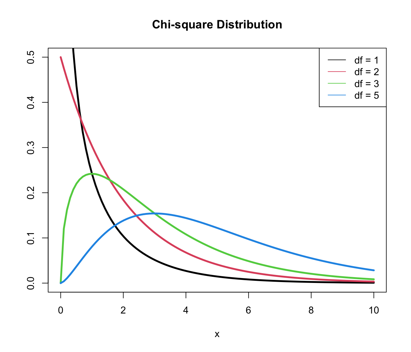
\(D \sim \chi^2_{n - p}\) ( \(D\) follows a Chi-square distribution with \(n - p\) degrees of freedom)³

Note: \(n - p\) a the degrees of freedom associated with the error in the model (like residuals)

\(\chi^2\) distribution

Test for overall significance

We can test the overall significance for a logistic regression model, i.e., whether there is at least one predictor with a non-zero coefficient

\[ \begin{aligned} &H_0: \beta_1 = \dots = \beta_p = 0 \\ &H_a: \beta_j \neq 0 \text{ for at least one } j \end{aligned} \]

The drop-in-deviance test for overall significance compares the fit of a model with no predictors to the current model.

Drop-in-deviance test statistic

Let \(L_0\) and \(L_a\) be the likelihood functions of the model under \(H_0\) and \(H_a\), respectively. The test statistic is

\[ \begin{aligned} G = D_0 - D_a &= (-2\log L_0) - (-2\log L_a)\\[5pt] & = -2(\log L_0 - \log L_a) \\[5pt] &= -2\sum_{i=1}^n \Big[ y_i \log \Big(\frac{\hat{\pi}^0}{\hat{\pi}^a_i}\Big) + (1 - y_i)\log \Big(\frac{1-\hat{\pi}^0}{1-\hat{\pi}^a_i}\Big)\Big] \end{aligned} \]

where \(\hat{\pi}^0\) is the predicted probability under \(H_0\) and \(\hat{\pi}_i^a = \frac{\exp \{x_i^\mathsf{T}\boldsymbol{\beta}\}}{1 + \exp \{x_i^\mathsf{T}\boldsymbol{\beta}\}}\) is the predicted probability under \(H_a\) ⁴

Drop-in-deviance test statistic

\[ G = -2\sum_{i=1}^n \Big[ y_i \log \Big(\frac{\hat{\pi}^0}{\hat{\pi}^a_i}\Big) + (1 - y_i)\log \Big(\frac{1-\hat{\pi}^0}{1-\hat{\pi}^a_i}\Big)\Big] \]

When \(n\) is large, \(G \sim \chi^2_p\), ( \(G\) follows a Chi-square distribution with \(p\) degrees of freedom)
The p-value is calculated as \(P(\chi^2 > G)\)
Large values of \(G\) (small p-values) indicate at least one \(\beta_j\) is non-zero

Heart disease model: drop-in-deviance test

\[ \begin{aligned} &H_0: \beta_{age} = \beta_{totChol} = \beta_{currentSmoker} = 0 \\ &H_a: \beta_j \neq 0 \text{ for at least one }j \end{aligned} \]

Fit the null model (we’ve already fit the alternative model)

null_model <- glm(high_risk ~ 1, data = heart_disease, family = "binomial")

term	estimate	std.error	statistic	p.value
(Intercept)	-1.72294	0.0436342	-39.486	0

Heart disease model: drop-in-deviance test

Calculate the log-likelihood for the null and alternative models

(L_0 <- glance(null_model)$logLik)

[1] -1737.735

(L_a <- glance(high_risk_fit)$logLik)

[1] -1612.406

Calculate the likelihood ratio test statistic

(G <- -2 * (L_0 - L_a))

[1] 250.6572

Heart disease model: likelihood ratio test

Calculate the p-value

(p_value <- pchisq(G, df = 3, lower.tail = FALSE))

[1] 4.717158e-54

Conclusion

The p-value is small, so we reject \(H_0\). The data provide evidence that at least one predictor in the model has a non-zero coefficient.

Why use overall test?

Why do we use a test for overall significance instead of just looking at the test for individual coefficients?⁵

Suppose we have a model such that \(p = 100\) and \(H_0: \beta_1 = \dots = \beta_{100} = 0\) is true

About 5% of the p-values for individual coefficients will be below 0.05 by chance.
So we expect to see 5 small p-values if even no linear association actually exists.
Therefore, it is very likely we will see at least one small p-value by chance.
The overall test of significance does not have this problem. There is only a 5% chance we will get a p-value below 0.05, if a relationship truly does not exist.

Test a subset of coefficients

Suppose there are two models:
- Reduced Model: includes predictors \(x_1, \ldots, x_q\)
- Full Model: includes predictors \(x_1, \ldots, x_q, x_{q+1}, \ldots, x_p\)
We can use a drop-in-deviance test to determine if any of the new predictors are useful

\[ \begin{aligned} &H_0: \beta_{q+1} = \dots = \beta_p = 0\\ &H_a: \beta_j \neq 0 \text{ for at least one }j \end{aligned} \]

The test statistic (drop-in deviance test) is

\[ \begin{aligned} G = D_{reduced} - D_{full} &= (-2\log L_{reduced}) - (-2 \log L_{full}) \\ &= -2(\log L_{reduced} - \log L_{full}) \end{aligned} \]

The p-value is calculated using a \(\chi_{\Delta df}^2\) distribution, where \(\Delta df\) is the number of parameters being tested (the difference in number of parameters between the full and reduced model).

Example: Include `education`?

Should we include education in the model?

Reduced model: age, totChol, currentSmoker
Full model: age, totChol, currentSmoker , education

\[ \begin{aligned} &H_0: \beta_{ed2} = \beta_{ed3} = \beta_{ed4} = 0 \\ &H_a: \beta_j \neq 0 \text{ for at least one }j \end{aligned} \]

reduced_model <- glm(high_risk ~ age + totChol + currentSmoker, 
              data = heart_disease, family = "binomial")

full_model <- glm(high_risk ~ age + totChol + currentSmoker + education, 
              data = heart_disease, family = "binomial")

Calculate deviances

(deviance_reduced <- -2 * glance(reduced_model)$logLik)

[1] 3224.812

(deviance_full <- -2 * glance(full_model)$logLik)

[1] 3217.6

Calculate test statistic

(G <- deviance_reduced - deviance_full)

[1] 7.212113

Calculate p-value

pchisq(G, df = 3, lower.tail = FALSE)

[1] 0.06543567

Exercise

What is your conclusion? Would you include education in the model that already has age, totChol, currentSmoker?

Drop-in-deviance test in R

Conduct the drop-in-deviance test using the anova() function in R with option test = "Chisq"

anova(reduced_model, full_model, test = "Chisq") |> 
  tidy() |> 
  kable(digits = 3)

term	df.residual	residual.deviance	df	deviance	p.value
high_risk ~ age + totChol + currentSmoker	4082	3224.812	NA	NA	NA
high_risk ~ age + totChol + currentSmoker + education	4079	3217.600	3	7.212	0.065

Add interactions with currentSmoker?

term	df.residual	residual.deviance	df	deviance	p.value
high_risk ~ age + totChol + currentSmoker	4082	3224.812	NA	NA	NA
high_risk ~ age + totChol + currentSmoker + currentSmoker * age + currentSmoker * totChol	4080	3222.377	2	2.435	0.296

Acknowledgements

Thanks to Prof. Maria Tackett for this example.

References

Footnotes

Akaike, Hirotugu. “A new look at the statistical model identification.” IEEE transactions on automatic control 19.6 (1974): 716-723.↩︎
Schwarz, Gideon. “Estimating the dimension of a model.” The annals of statistics (1978): 461-464.↩︎
See @wilks1935likelihood for explanation of why -2 is included.↩︎
See @wilks1935likelihood for explanation of why -2 is included.↩︎
Example from Introduction to Statistical Learning↩︎

Topics

Risk of coronary heart disease

Model comparison

Which model do we choose?

Log-Likelihood

AIC & BIC

AIC & BIC

AIC & BIC

Using AIC & BIC

AIC from the glance() function

Comparing the models using AIC

Comparing the models using BIC

Drop-in-deviance test

Drop-in-deviance test

Deviance

\(\chi^2\) distribution

Test for overall significance

Drop-in-deviance test statistic

Drop-in-deviance test statistic

Heart disease model: drop-in-deviance test

Heart disease model: drop-in-deviance test

Heart disease model: likelihood ratio test

Why use overall test?

Test a subset of coefficients

Example: Include education?

Drop-in-deviance test in R

Acknowledgements

References

Footnotes

AIC from the `glance()` function

Example: Include `education`?