library(tidyverse)library(tidymodels)library(pROC) # make ROC curveslibrary(knitr)library(kableExtra)## data heart_disease <-read_csv("https://sta221-fa25.github.io/data/framingham.csv") |>select(age, totChol, TenYearCHD, currentSmoker) |>drop_na() |>mutate(high_risk =as_factor(TenYearCHD), currentSmoker =as_factor(currentSmoker))# set default theme in ggplot2ggplot2::theme_set(ggplot2::theme_bw())
Topics
Calculating predicted probabilities from the logistic regression model
Using predicted probabilities to classify observations
Make decisions and assess model performance using
Confusion matrix
ROC curve
Data: Risk of coronary heart disease
This data set is from an ongoing cardiovascular study on residents of the town of Framingham, Massachusetts. We want to examine the relationship between various health characteristics and the risk of having heart disease.
high_risk: 1 = High risk of having heart disease in next 10 years, 0 = Not high risk of having heart disease in next 10 years
age: Age at exam time (in years)
totChol: Total cholesterol (in mg/dL)
currentSmoker: 0 = nonsmoker; 1 = smoker
Modeling risk of coronary heart disease
heart_disease_fit <-glm(high_risk ~ age + totChol + currentSmoker, data = heart_disease, family ="binomial")tidy(heart_disease_fit, conf.int =TRUE) |>kable(digits =3)
Interpret currentSmoker1 in terms of the odds of being high risk for heart disease.
Interpret totChol in terms of the odds of being high risk for heart disease.
The odds of being high risk for heart disease for smokers is expected to be \(\exp\{\hat{\beta}_{smoker}\} = \exp\{0.457\} =\) 1.579 times the odds of a non-smoker being high risk for heart disease, holding all else constant.
The odds of being high risk for heart disease increases multiplicatively, by a factor of \(\exp\{\hat{\beta}_{totChol}\} = \exp\{0.002\} =\) 1.002 for each unit increase in total cholestorol.
Prediction and classification
We are often interested in using the model to classify observations, i.e., predict whether a given observation will have a 1 or 0 response
For each observation
Use the logistic regression model to calculate the predicted log-odds the response for the \(i^{th}\) observation is 1
Use the log-odds to calculate the predicted probability the \(i^{th}\) observation is 1
Then, use the predicted probability to classify the observation as having a 1 or 0 response using some predefined threshold
A confusion matrix is a \(2 \times 2\) table that compares the predicted and actual classes. We can produce this matrix using the conf_mat() function in the yardstick package (part of tidymodels).
A doctor plans to use your model to determine which patients are high risk for heart disease. The doctor will recommend a treatment plan for high risk patients.
Would you want sensitivity to be high or low? What about specificity?
What are the trade-offs associated with each decision?
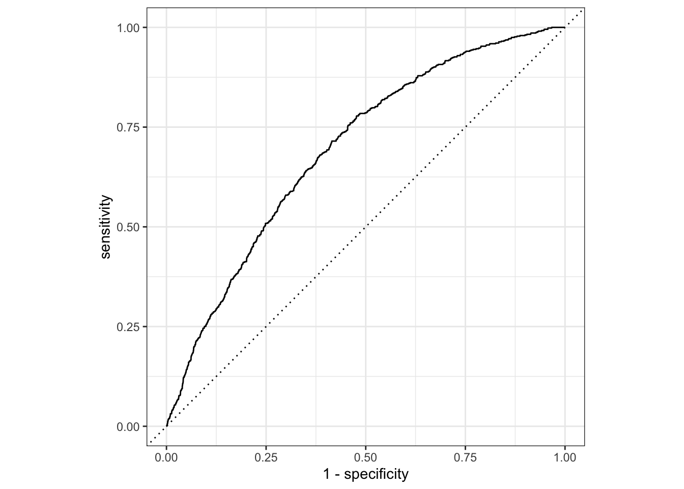
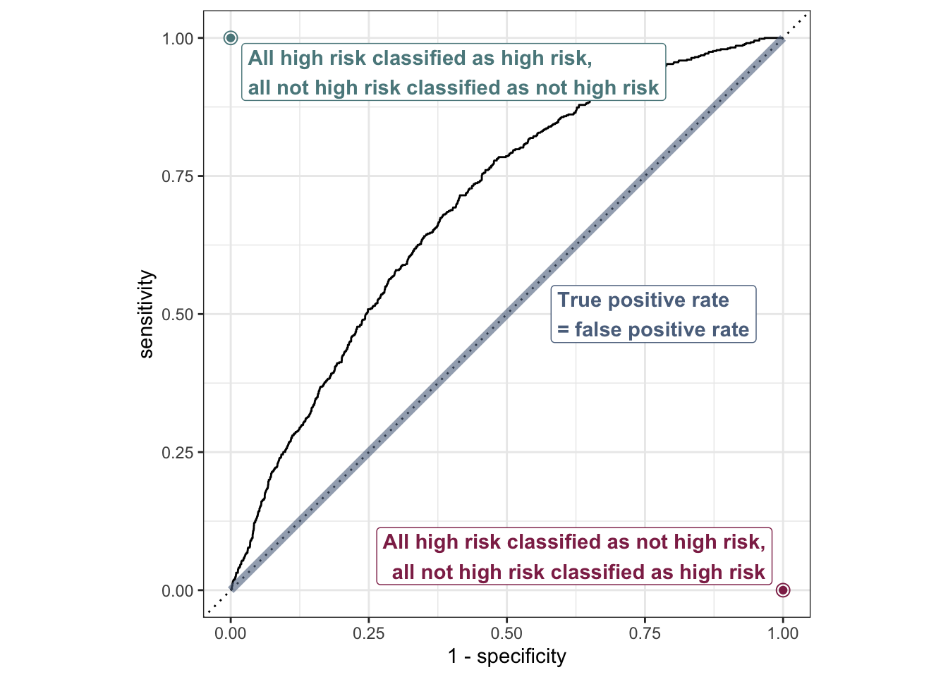
ROC curve
So far the model assessment has depended on the model and selected threshold. The receiver operating characteristic (ROC) curve allows us to assess the model performance across a range of thresholds.
x-axis: 1 - Specificity (False positive rate)
y-axis: Sensitivity (True positive rate)
Which corner of the plot indicates the best model performance?
ROC curve
ROC curve in R
# calculate sensitivity and specificity at each thresholdroc_curve_data <- heart_disease_aug |>roc_curve(high_risk, pred_prob, event_level ="second") # event_level = second binary outcome is "1" outcome# plot roc curveautoplot(roc_curve_data)
This data consists of 4601 emails that are classified as spam or non-spam. The data was collected at Hewlett-Packard labs and contains 58 variables. The first 48 variables are specific keywords and each observation is the percentage of appearance (frequency) of that word in the message. Click here to read more.
newEmailText ="CONGRATULATIONS!!! YOU have been selected as one of our lucky winners to receive a $0.5 Amazon Gift Card.To claim your reward, simply click the link below and confirm your details.Claim Your Gift Now"
Footnotes
The default is type = "link", which produces the predicted log-odds.↩︎