Intro to logistic regression

Author

Dr. Alexander Fisher

View libraries and data used in these notes

library(tidyverse)
library(tidymodels)

orings = read_csv("https://sta221-fa25.github.io/data/orings.csv")

Data: O-ring example

In January 1986, the space shuttle Challenger exploded 73 seconds after launch.
The culprit is the O-ring seals in the rocket boosters. At lower temperatures, rubber becomes more brittle and is a less effective sealant. At the time of the launch, the temperature was 31°F.
Could the failure of the O-rings have been predicted?
Data: 23 previous shuttle missions. Each shuttle had 2 boosters, each with 3 O-rings. We know whether or not at least one of the O-rings was damaged and the launch temperature.

orings %>%
  print(n = Inf)

# A tibble: 23 × 3
   mission  temp damage
     <dbl> <dbl>  <dbl>
 1       1    53      1
 2       2    57      1
 3       3    58      1
 4       4    63      1
 5       5    66      0
 6       6    67      0
 7       7    67      0
 8       8    67      0
 9       9    68      0
10      10    69      0
11      11    70      1
12      12    70      0
13      13    70      1
14      14    70      0
15      15    72      0
16      16    73      0
17      17    75      0
18      18    75      1
19      19    76      0
20      20    76      0
21      21    78      0
22      22    79      0
23      23    81      0

Descriptive statistics

Notice any patterns?

orings %>%
  mutate(failrate = damage) %>%
  ggplot(mapping = aes(x = temp, y = failrate)) + 
  geom_point() + 
  labs(x = "Temperature (F)", y = "Damage to O-rings", title = "O-ring damage data") +
  theme_bw()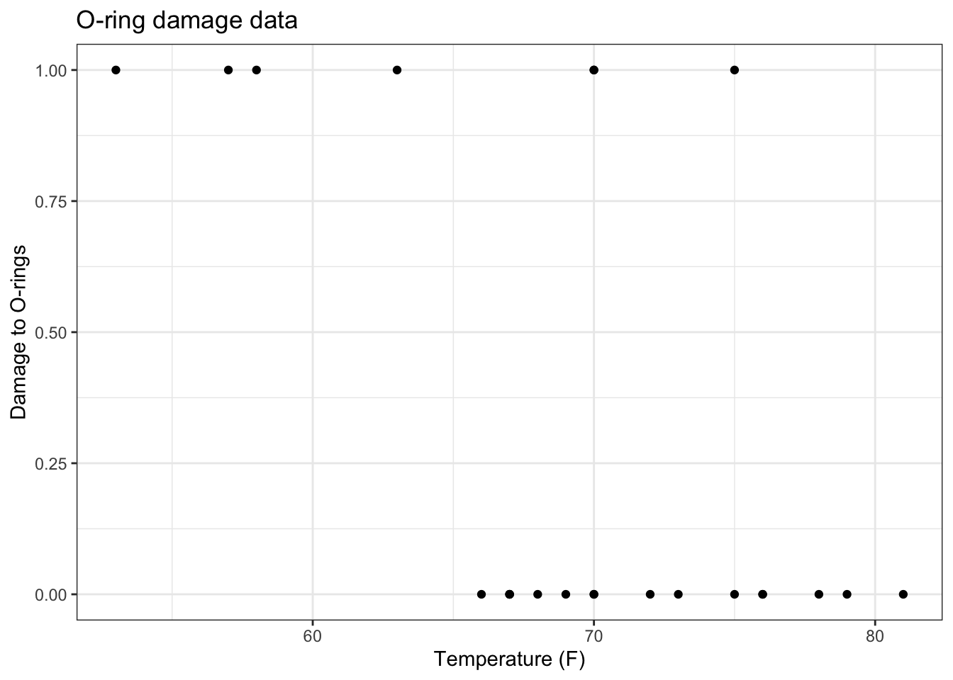

Question
Does this make sense?

Can we fit a linear model?

orings %>%
  mutate(failrate = damage) %>%
  ggplot(mapping = aes(x = temp, y = failrate)) + 
  geom_point() + 
  labs(x = "Temperature (F)", y = "Damage to O-rings", title = "O-ring damage data") +
  theme_bw() +
  geom_smooth(method = lm, se = FALSE, color = "steelblue")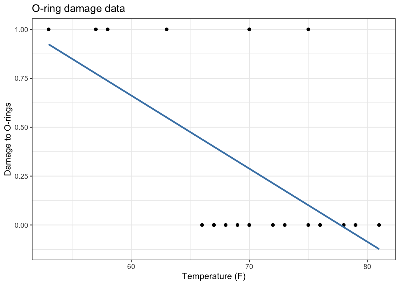

Binary outcome model

We model each outcome \(Y_i\) as a binary random variable. The probability \(Y_i\) takes the value 1 is \(p\).

\[ \begin{aligned} Prob(Y_i = 1) &= p\\ Prob(Y_i = 0) &= (1-p) \end{aligned} \]

Exercise
Solution

What is \(E[Y_i|p]\)?

\[ \begin{aligned} E[Y_i|p] &= \sum_{Y_i = 0}^1 Y_i \cdot prob(Y_i)\\ &= 0 \cdot prob(Y_i = 0) + 1 \cdot prob(Y_i = 1)\\ &= 0 \cdot (1-p) + 1 \cdot p\\ &= p \end{aligned} \]

In linear regression, we are concerned with modeling the conditional expectation of the outcome variable. (Previously: \(E[y|X] = X\beta\)).
Here, the conditional expectation \(E[Y_i | p] = p\).

Exercise
Solution

If \(p = 0.5\), what does the statemeny \(E[Y_i | p] = p\) say, in terms of the data at hand? Is this assumption realistic?

That the probability of O-ring failure is 0.5 for all observations.
Not realistic given EDA above.
We want to have individual observation probabilities \(p_i\) that depends on the covariate temperature.

What’s wrong with letting \(p_i = x_i \beta\)?

\(p_i\) is bounded between \([0, 1]\), \(x_i \beta\) is not. See figure above again.

Remedy: let

\[ \text{logit}(p_i) = x_i^T\beta \]

where \(\text{logit}(p_i) = \log \frac{p_i}{1-p_i}\). Since the logit function links our conditional expectation to the predictor(s), we call the logit function a link function.

Exercise

What happens as \(p_i \rightarrow 0\)?

What happens as \(p_i \rightarrow 1\)?

We can solve for \(p_i\) directly:

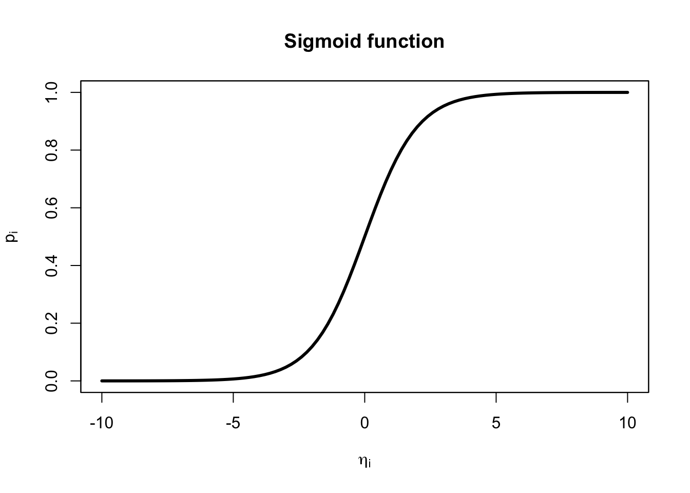
\[ p_i = \frac{e^{\eta_i}}{1 + e^{\eta_i}} = \frac{1}{e^{-\eta_i}+ 1}, \]

where the second equality comes from multiplying by 1 in a fancy way: \(\frac{e^{-\eta_i}}{e^{-\eta_i}}\) and \(\eta_i = x_i^T\beta = \beta_0 + \beta_1 x_1 + \ldots\) is called the linear predictor or systematic component.

\[ \eta_i = \beta_0 + \beta_1 x_{i1} + \cdots + \beta_{q} x_{iq} = \mathbf{x}_i^T \boldsymbol{\beta} \] The function \(p_i = \frac{e^{\eta_i}}{1 + e^{\eta_i}}\) has a special name. It is called a “sigmoid” function. Let’s take a look at the sigmoid function:

The likelihood

Here’s our model:

\[ E[Y_i | X] = p_i = \frac{1}{e^{-x_i^T\beta}+ 1} \]

The likelihood of the data is the joint density of the data, viewed as a function of the unknown parameters:

\[ \begin{aligned} \underbrace{p(y_1, \ldots, y_n| X, \beta)}_{\text{joint density of data}} &= \prod_{i=1}^n p(y_i|X, \beta)\\ &= \prod_{i=1}^np_i^{y_i} (1-p_i)^{1-y_i} \end{aligned} \]

Practically, we want to examine the log-likelihood for numerical stability. Recall: maximizing the log-likelihood (finding \(\hat{\beta}_{MLE}\)) will be the same as maximizing the likelihood since \(\log()\) is a monotonic function.

\[ \begin{aligned} \log p(y_1, \ldots, y_n | X,\beta) &= \sum_{i=1}^n y_i \log(p_i) + (1-y_i) \log(1 - p_i) \end{aligned} \] Plugging in \(p_i\), we view the log-likelihood as a function of the unknown parameter vector \(\beta\), and we can simplify:

\[ \begin{aligned} \log L(\beta) &= \sum_{i=1}^n y_i \log \left(\frac{e^{x_i^T\beta}}{1 + e^{x_i^T\beta}} \right) + (1-y_i) \log \left(\frac{1}{1 + e^{x_i^T\beta}} \right)\\ &= \sum_{i=1}^n y_i x_i^T \beta - \sum_{i=1}^n \log(1+ \exp\{x_i^T \beta\}) \end{aligned} \]

Finding the MLE

Taking the derivative:

\[ \begin{aligned} \frac{\partial \log L}{\partial \boldsymbol\beta} =\sum_{i=1}^n y_i x_i^\top &- \sum_{i=1}^n \frac{\exp\{x_i^\top \boldsymbol\beta\} x_i^\top}{1+\exp\{x_i^\top \boldsymbol\beta\}} \end{aligned} \]

If we set this to zero, there is no closed form solution.
R uses numerical approximation to find the MLE.

Logistic regression in R

orings_fit = glm(damage ~ temp, 
                         data  = orings, 
                         family = "binomial")

summary(orings_fit)


Call:
glm(formula = damage ~ temp, family = "binomial", data = orings)

Coefficients:
            Estimate Std. Error z value Pr(>|z|)  
(Intercept)  15.0429     7.3786   2.039   0.0415 *
temp         -0.2322     0.1082  -2.145   0.0320 *
---
Signif. codes:  0 '***' 0.001 '**' 0.01 '*' 0.05 '.' 0.1 ' ' 1

(Dispersion parameter for binomial family taken to be 1)

    Null deviance: 28.267  on 22  degrees of freedom
Residual deviance: 20.315  on 21  degrees of freedom
AIC: 24.315

Number of Fisher Scoring iterations: 5

Prediction

Now we can predict the failure probability. The failure probability at 31F is nearly 1.

test_31F = tibble(temp     = seq(25, 85, 0.1), 
       predprob = predict(orings_fit, newdata = tibble(temp = temp), type = "response"))

test_31F %>%
  ggplot() + 
  geom_line(mapping = aes(x = temp, y = predprob)) + 
  geom_vline(xintercept = 31) +
  labs(x = "Temperature (F)", y = "Predicted failure probability") +
  theme_bw()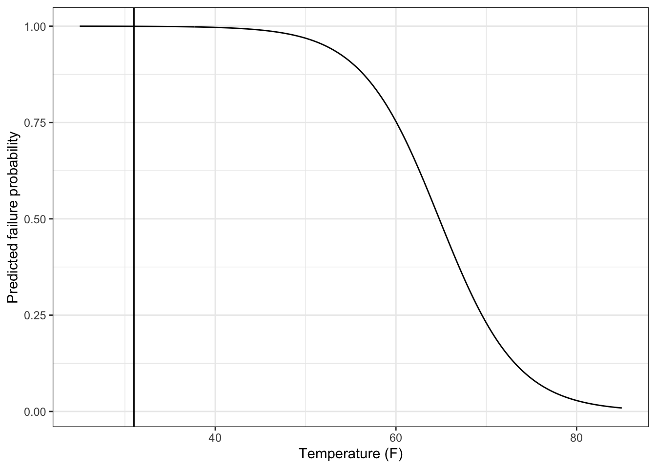

# make augmented model fit
orings_aug = 
  augment(orings_fit)

# add to the augmented model fit a column for 
# predicted probability
orings_aug$predicted_prob = 
  predict.glm(orings_fit, orings, type = "response")

orings_aug %>%
  mutate(y = damage) %>%
  select(predicted_prob, .fitted, y) %>%
  head(5)

# A tibble: 5 × 3
  predicted_prob .fitted     y
           <dbl>   <dbl> <dbl>
1          0.939   2.74      1
2          0.859   1.81      1
3          0.829   1.58      1
4          0.603   0.417     1
5          0.430  -0.280     0

predicted_prob: predicted probability that \(Y_i = 1\), i.e. \(\hat{p}_i\)
.fitted: predicted log-odds, i.e. \(\log \left(\frac{\hat{p_i}}{1 - \hat{p}_i}\right)\).
y: actual outcome

Acknowledgements

Thanks to Prof. Hua Zhou for example.