Generalized Least Squares: R example

library(tidyverse)
library(tidymodels)
library(nlme) # package for GLS, AR1 model
library(mvtnorm) # for density of a multivariate normal

load(url("https://sta221-fa25.github.io/data/VostokIce"))

Data

Vostok station is a Russian research station founded by the Soviet Union in 1957. The station is near the South Pole in Antarctica and has recorded the lowest reliably measured natural temperature on Earth (-89.2 C or -128.6 F). The station sits on an ice sheet. The ice-core project had researchers drill over 3500 meters in below the surface of the ice sheet to retrieve “ice cores”. The ice cores provide us with a few pieces of data.

• year: scientists estimate “years before present” at which ice was frozen by counting layers of ice (by assuming some constants, such as regularity of snow, etc.)

• co2: atmospheric \(CO_2\) concentration (ppm), preserved in the ice within trapped air bubbles.

• tmp: a measure of past temperature, recorded as a difference from current and constructed from based on the isotopes of \(CO_2\) found. The key idea being that colder temperatures result in fewer heavy isotopes during snowfall.

glimpse(VostokIce)

Rows: 200
Columns: 3
$ year <dbl> -419095, -416872, -414692, -413062, -410979, -408485, -406441, -4…
$ co2  <dbl> 277.6, 286.9, 285.5, 285.5, 281.2, 281.2, 279.7, 279.7, 278.0, 27…
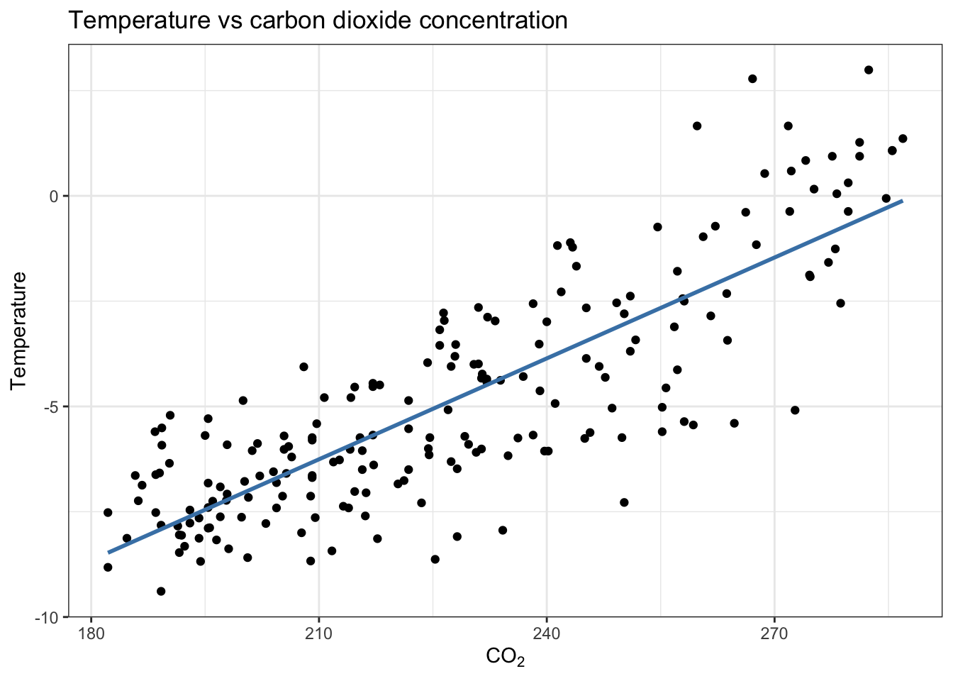
$ tmp  <dbl> 0.94, 1.36, 1.07, 1.08, 1.27, 0.94, 0.31, -0.37, -1.26, -1.58, -1…

Motivating question

Can temperature be explained by \(CO_2\) concentration in the atmosphere?

EDA

Plot

Code

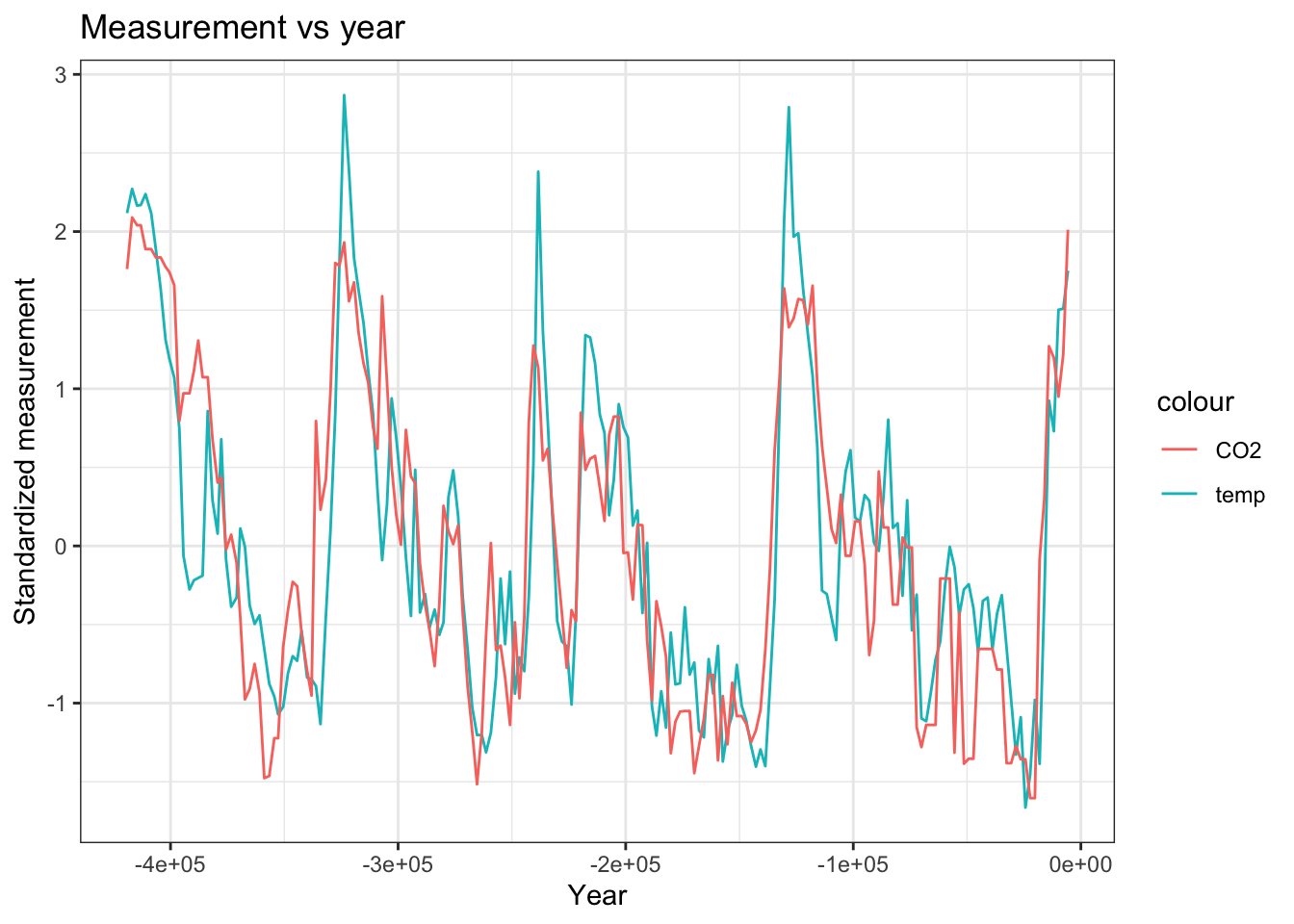
VostokIce %>%
  mutate(tmpStd = ((tmp - mean(tmp)) / sd(tmp))) %>%
  mutate(co2Std = (co2 - mean(co2)) / sd(co2)) %>%
  ggplot(aes(x = year, y = tmpStd)) + 
  theme_bw() +
  geom_line(aes(col = "temp")) +
  geom_line(aes(x = year, y = co2Std, col = "CO2"),) +
  labs(x = "Year", y = "Standardized measurement", title = "Measurement vs year")

Fit model

fit = lm(tmp ~ co2, data = VostokIce)
summary(fit) %>%
  tidy()

# A tibble: 2 × 5
  term        estimate std.error statistic  p.value
  <chr>          <dbl>     <dbl>     <dbl>    <dbl>
1 (Intercept) -23.0      0.880       -26.2 3.27e-66
2 co2           0.0799   0.00383      20.8 8.77e-52

Check assumptions

fit_aug = augment(fit)

ggplot(data = fit_aug, aes(x = .fitted, y = .resid)) +
  geom_point() + 
  geom_hline(yintercept = 0, linetype = 2, color = "red") + 
  labs(x = "Fitted values", 
       y = "Residuals", 
       title = "Residuals vs. Fitted Values") +
  theme_bw()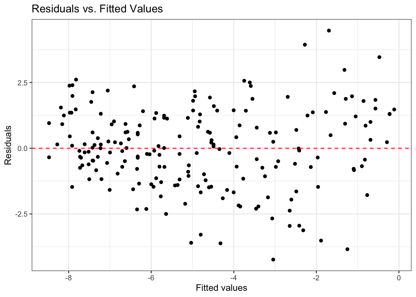

ggplot(fit_aug, aes(sample = .std.resid)) +
  stat_qq() +
  stat_qq_line() +
  labs(title = "Normal Q-Q Plot of Standardized Residuals",
       x = "Theoretical Quantiles",
       y = "Standardized Residuals") +
  theme_minimal()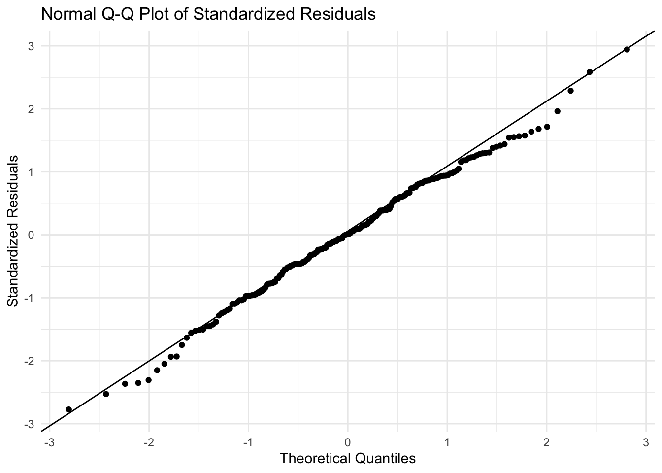

A Q–Q (quantile–quantile) plot compares the quantiles of your residuals to those of a theoretical distribution (in this case a normal). If the points fall roughly along a straight line, the residuals follows a normal distribution closely.

Checking residuals in time

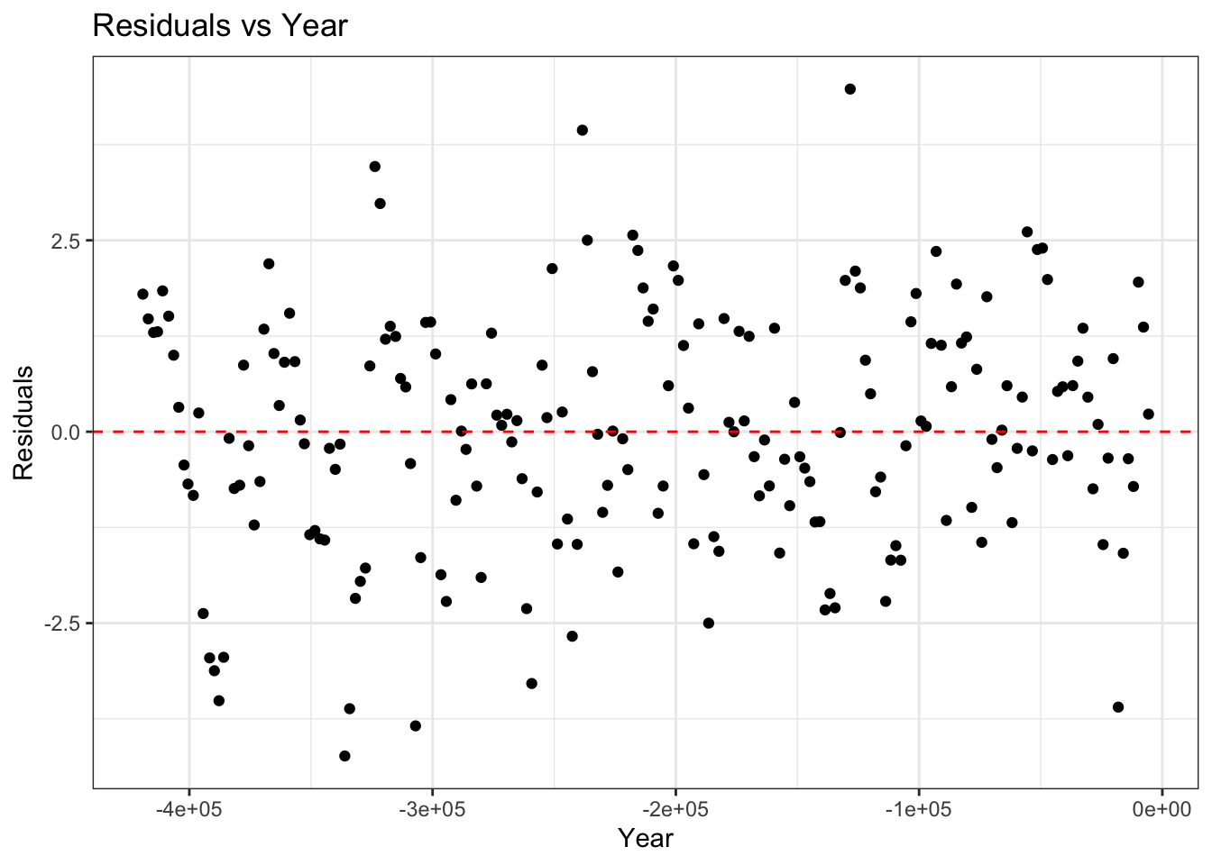
fit_aug %>%
  mutate(year = VostokIce$year) %>%
ggplot( aes(x = year, y = .resid)) +
  geom_point() +
  geom_line() +
  geom_hline(yintercept = 0, linetype = "dashed", color = "red") +
  labs(
    x = "Year",
    y = "Residuals",
    title = "Residuals vs Year"
  ) +
  theme_bw()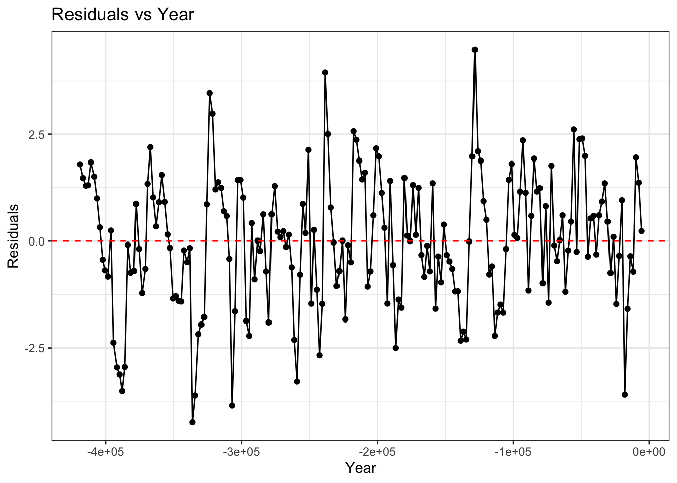

Evidence of lag-1 correlation

Quick look

auto_correlation = acf(fit$residuals)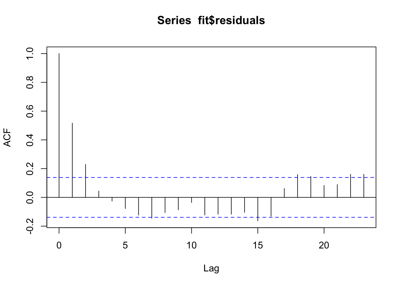

auto_correlation$acf[2] # lag-1 (first entry = lag-0)

[1] 0.5165516

Manual look

res_t1 = fit$res[-1] # residuals minus the first.
res_t0 = fit$res[-length(fit$res)] # residuals minus the last
resid_matrix = cbind(res_t0 , res_t1 ) # combine the two
resid_matrix[1:4,]

    res_t0   res_t1
1 1.796974 1.474342
2 1.474342 1.296136
3 1.296136 1.306136
4 1.306136 1.839503

cor(resid_matrix) # correlation between residuals

          res_t0    res_t1
res_t0 1.0000000 0.5183877
res_t1 0.5183877 1.0000000

Generalized least squares

Using nlme package

Before fitting with an AR1 model, we sort the data frame by year.

# Step (1): sort by time
# This matters since we don't explicitly give the "year 
# variable" a place in the AR1 model below
VostokIce = VostokIce %>%
  arrange(year)

# Auto-regressive lag-1 model:
fit_gls_ar1 = gls(
  tmp ~ co2,
  data = VostokIce,
  correlation = corAR1(form = ~ 1), 
  method = "ML" # maximum likelihood
)
summary(fit_gls_ar1)

Generalized least squares fit by maximum likelihood
  Model: tmp ~ co2 
  Data: VostokIce 
       AIC      BIC    logLik
  657.3112 670.5045 -324.6556

Correlation Structure: AR(1)
 Formula: ~1 
 Parameter estimate(s):
      Phi 
0.8284176 

Coefficients:
                 Value Std.Error   t-value p-value
(Intercept) -10.860283 1.6908246 -6.423069   0e+00
co2           0.027201 0.0070254  3.871772   1e-04

 Correlation: 
    (Intr)
co2 -0.956

Standardized residuals:
       Min         Q1        Med         Q3        Max 
-1.7849930 -0.7876546 -0.3111786  0.5258292  2.9192183 

Residual standard error: 2.18379 
Degrees of freedom: 200 total; 198 residual

Manual fit

Direct formula

n = nrow(VostokIce)
rho = coef(fit_gls_ar1$modelStruct$corStruct, unconstrained = FALSE) 
Sigma = rho ^ abs(outer(1:n, 1:n, "-")) # construct Sigma
X = model.matrix(~ co2, data = VostokIce)
y = VostokIce$tmp
beta_hat = solve(t(X) %*% solve(Sigma) %*% X) %*% t(X) %*% solve(Sigma) %*% y
beta_hat

                    [,1]
(Intercept) -10.86028298
co2           0.02720076

Exercise

Do we need to know \(\sigma^2\) the scalar multiple of our covariance matrix to compute \(\hat{\beta}_{GLS}\)?

Solution

No, let \(\Sigma = \sigma^2 A\) to see this:

\[ \begin{aligned} \hat{\beta}_{GLS} &= (X^T \Sigma^{-1} X)^{-1} X^T \Sigma^{-1}y\\ &= (X^T (\sigma^2 A)^{-1} X)^{-1} X^T (\sigma^2 A)^{-1} y\\ &= \sigma^2(X^T A^{-1}X)^{-1} X^T \frac{1}{\sigma^2} A^{-1}y\\ &= (X^T A^{-1}X)^{-1} X^T A^{-1}y \end{aligned} \]

Using lm

E = eigen(Sigma, symmetric = TRUE)
V = E$vectors

Sigma_invhalf = V %*% diag(1 / sqrt(E$values)) %*% t(V) # Sigma^{-1/2}

ystar = Sigma_invhalf %*% y
Xstar = Sigma_invhalf %*% X

# Note: X already contains intercept, so lm(y ~ 0 + X)
fit_gls = lm(ystar ~ 0 + Xstar)
summary(fit_gls)

Call:
lm(formula = ystar ~ 0 + Xstar)

Residuals:
    Min      1Q  Median      3Q     Max 
-5.9697 -1.5481 -0.2285  1.3725  9.4874 

Coefficients:
                   Estimate Std. Error t value Pr(>|t|)    
Xstar(Intercept) -10.860283   1.690825  -6.423 9.71e-10 ***
Xstarco2           0.027201   0.007025   3.872 0.000147 ***
---
Signif. codes:  0 '***' 0.001 '**' 0.01 '*' 0.05 '.' 0.1 ' ' 1

Residual standard error: 2.195 on 198 degrees of freedom
Multiple R-squared:  0.3387,    Adjusted R-squared:  0.3321 
F-statistic: 50.71 on 2 and 198 DF,  p-value: < 2.2e-16

Computing log-likelihood manually

s2 = sigma(fit_gls_ar1)^2
X = model.matrix(tmp ~ co2, data = VostokIce)
logLikelihood = dmvnorm(y, mean = X %*% beta_hat, s2 * Sigma, log = TRUE)
logLikelihood

[1] -324.6556

fit_gls_ar1$logLik

[1] -324.6556

Computing AIC manually

# Compute AIC directly:
c = 2 
-2 * fit_gls_ar1$logLik + (4 * c)

[1] 657.3112

AIC(fit_gls_ar1)

[1] 657.3112

Exercise

Why is p = 4 used for the AIC calculation?

Solution

\(\beta_0, \beta_1, \sigma^2, \rho\) are all unknown parameters in the likelihood.