MLEs and Model Comparison

Author

Dr. Alexander Fisher

View libraries and data used in these notes
library(tidyverse)
library(GGally)
library(corrplot)
library(tidymodels)
nba_salaries <- 
  read_csv("https://sta221-fa25.github.io/data/nba_salaries_23.csv") %>%
  mutate(Salary = Salary / 1E6) %>% # salary in millions
  select(`Player Name`, Salary, Position, Age, GP, MP, GS, 
         FG, `FG%`, `2PA`, `2P%`, AST, `AST%`) %>%
  filter(Position %in% c("SG", "C", "SF", "PF", "PG" )) %>%
  drop_na()

Topics

  • Properties of MLEs
  • Model selection via information criteria (AIC, BIC)

Recap

Linear regression statistical model:

\[ \boldsymbol{y}| \boldsymbol{X}\sim N_n(\boldsymbol{X}\beta, \sigma^2 \boldsymbol{I}) \] where \(\boldsymbol{y}\in \mathbb{R}^n\) and \(\boldsymbol{X}\in \mathbb{R}^{n \times p}\). Here \(N_n\) means “multivariate normal of dimension n”.

Therefore, the likelihood (joint density of the data, viewed as a function of the parameters) is

\[ L(\beta, \sigma^2) = (2\pi \sigma^2)^{-n/2} \exp\{ -\frac{1}{2\sigma^2} (\boldsymbol{y}- \boldsymbol{X}\beta)^T (\boldsymbol{y}- \boldsymbol{X}\beta)\} \]

Where does the likelihood expression come from? Identify which component of the likelihood is the RSS.

We can arrive at this likelihood using the multivariate normal density function. \(\boldsymbol{y}\sim N_n(\boldsymbol{\mu}, \Sigma)\) means that its density can be written,

\[ f_Y(\boldsymbol{y}) = (2 \pi)^{-n/2} |\Sigma|^{-1/2} \exp \{ (\boldsymbol{y}- \boldsymbol{\mu})^T \Sigma^{-1} (\boldsymbol{y}- \boldsymbol{\mu})\} \]

Notice the diagonal covariance matrix in the multivariate normal representation. We could equivalently write the model as \(y_i \sim N(x_i^T \beta, \sigma^2)\) and write the joint density as

\[ f(y_1, \ldots, y_n | x_1, \ldots, x_n) = \prod_{i=1}^n f_y(y_i|x_i) \] where \(f(y_i | x_i) = (2 \pi \sigma^2)^{-1/2} \exp\{ - \frac{1}{2\sigma^2} (y_i - x_i^T \beta)^2\}\) and arrive at the same likelihood function of \(\beta\) and \(\sigma^2\).

Question: Is a likelihood a density function of the parameters?

Answer: NO!

Maximum likelihood estimates

Maximum likelihood estimates are obtained by calculus: differentiate the likelihood function and set equal to zero.

Doing so, we find:

\[ \begin{aligned} \hat{\beta}_{MLE} &= (\boldsymbol{X}^T \boldsymbol{X})^{-1} \boldsymbol{X}^T \boldsymbol{y}= \hat{\beta}_{OLS}\\ \hat{\sigma^2}_{MLE} &= \frac{RSS}{n} \end{aligned} \]

Properties of maximum likelihood estimators

Maximum likelihood estimators have nice properties:

  1. Asymptotic consistency
  2. Asymptotic efficiency
  3. Asymptotic normality

Asymptotic consistency

Definition

Given a sequence of estimators, \(\hat{\theta}_1, \hat{\theta}_2, \ldots\), we say \(\hat{\theta}_n\) is a consistent estimator of \(\theta\) if for all \(c>0\),

\[ \lim_{n \rightarrow \infty} p(|\hat{\theta}_n - \theta| \geq c) = 0 \]

Meaning: as sample size \(n \rightarrow \infty\), the estimator will be arbitrarily close to the parameter with high probability.

Equivalently, an estimator \(\hat{\theta_n}\) is consistent if

\[ \begin{aligned} \lim_{n \rightarrow \infty} \text{var}(\hat{\theta}) &= 0\\ \lim_{n \rightarrow \infty} \text{bias}(\hat{\theta}) &= 0 \end{aligned} \]

Asymptotic efficiency

Definition: efficient

An estimator is efficient if it has the smallest variance among a class of estimators.

  • Gauss Markov theorem showed \(\hat{\beta}_{OLS}\) is the most efficient among all linear unbiased estimators (see homework 2).

  • MLEs are asymptotically efficient.

Asymptotically normal

As \(n \rightarrow \infty\), maximum likelihood estimators are asymptotically normal. This means that the distribution of \(\hat{\beta}_{MLE}\) is normal when \(n\) is large regardless of the distribution of the underlying data.

Model selection (by example)

Data

Data on NBA player salaries and metrics for the 2022-2023 season. Data sourced from kaggle but originally scraped from “Hoopshype” and “Basketball Reference”.

We’ll look at a subset of the data below.

glimpse(nba_salaries)
Rows: 456
Columns: 13
$ `Player Name` <chr> "Stephen Curry", "John Wall", "Russell Westbrook", "LeBr…
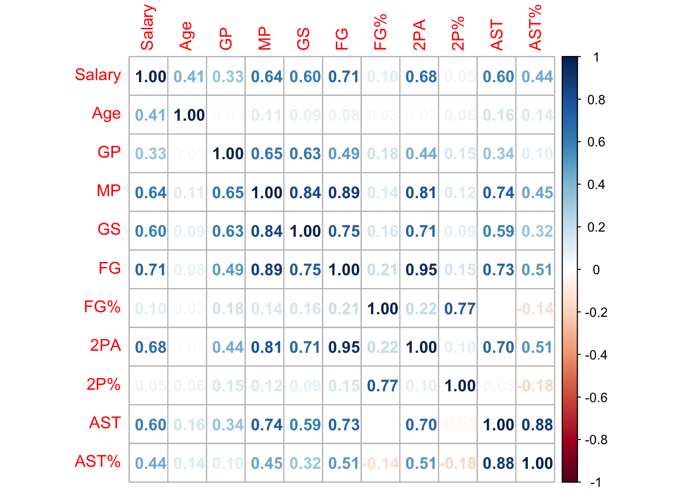
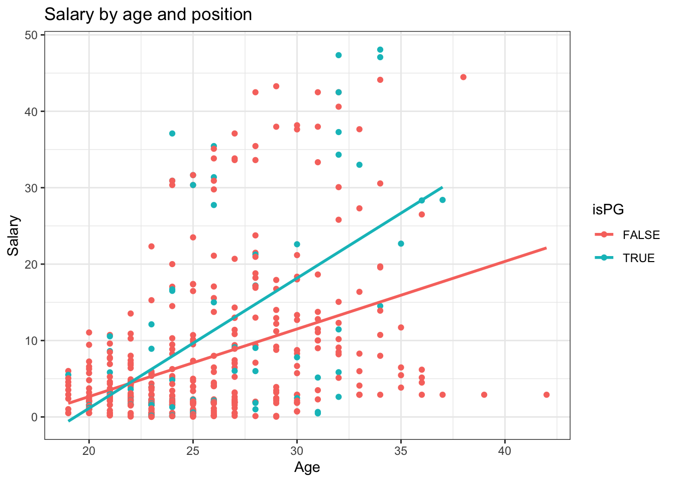
$ Salary        <dbl> 48.07001, 47.34576, 47.08018, 44.47499, 44.11984, 43.279…
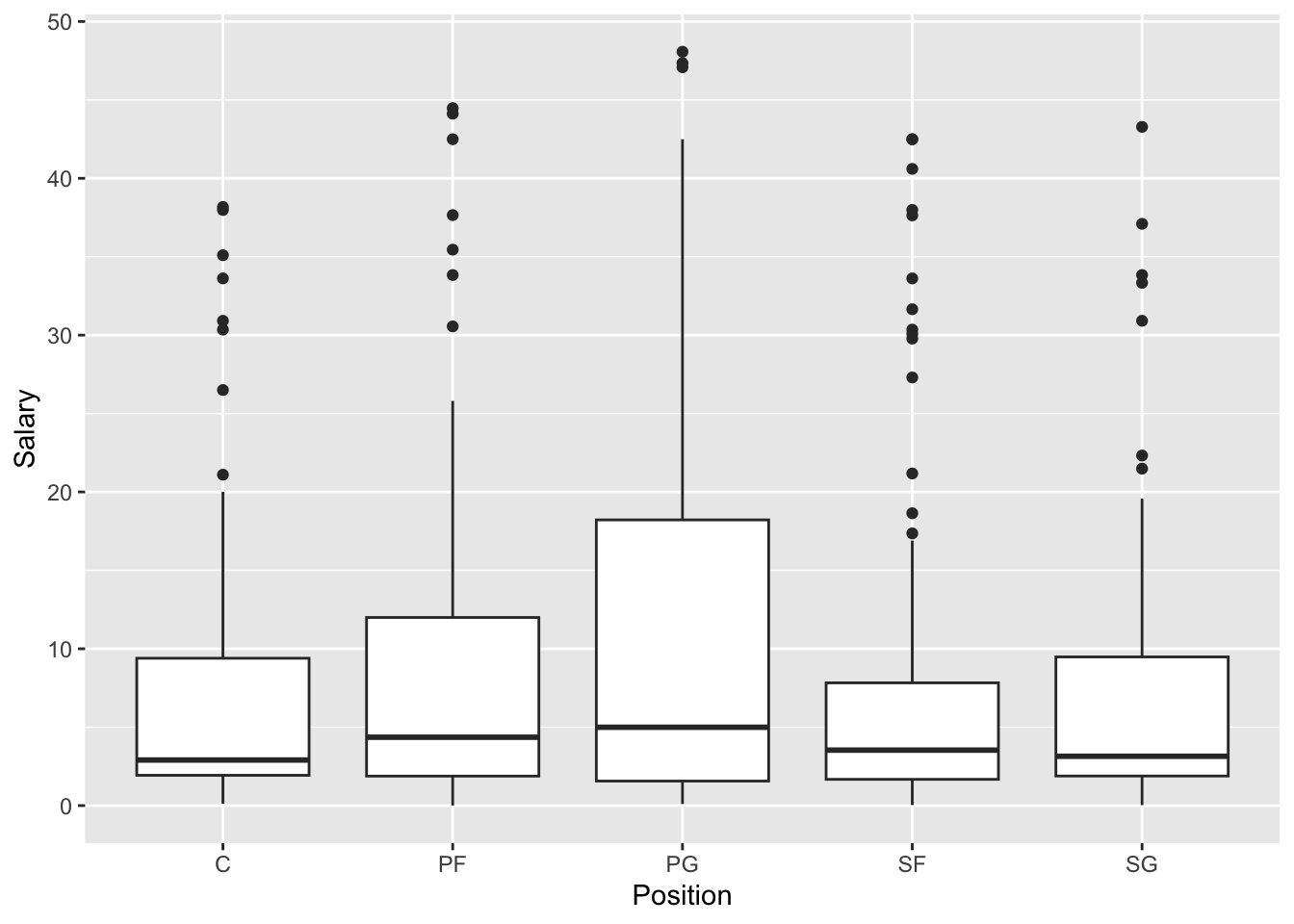
$ Position      <chr> "PG", "PG", "PG", "PF", "PF", "SG", "SF", "SF", "PF", "P…
$ Age           <dbl> 34, 32, 34, 38, 34, 29, 31, 32, 28, 32, 32, 30, 31, 29, …
$ GP            <dbl> 56, 34, 73, 55, 47, 50, 52, 56, 63, 58, 69, 70, 33, 56, …
$ MP            <dbl> 34.7, 22.2, 29.1, 35.5, 35.6, 33.5, 33.6, 34.6, 32.1, 36…
$ GS            <dbl> 56, 3, 24, 54, 47, 50, 50, 56, 63, 58, 69, 70, 19, 54, 6…
$ FG            <dbl> 10.0, 4.1, 5.9, 11.1, 10.3, 8.9, 8.6, 8.2, 11.2, 9.6, 7.…
$ `FG%`         <dbl> 0.493, 0.408, 0.436, 0.500, 0.560, 0.506, 0.512, 0.457, …
$ `2PA`         <dbl> 8.8, 6.7, 9.7, 15.3, 13.4, 13.2, 11.9, 10.3, 17.6, 9.4, …
$ `2P%`         <dbl> 0.579, 0.459, 0.487, 0.580, 0.617, 0.552, 0.551, 0.521, …
$ AST           <dbl> 6.3, 5.2, 7.5, 6.8, 5.0, 5.4, 3.9, 5.1, 5.7, 7.3, 2.4, 1…
$ `AST%`        <dbl> 30.0, 35.3, 38.6, 33.5, 24.5, 26.6, 19.6, 24.2, 33.2, 35…

Codebook

  • Salary: salary in millions of US dollars
  • Position: player position
  • Age: age of player
  • GP: total number of games played in the season
  • MP: average minutes played per game
  • GS: number of games the player is put in at the start of the game
  • FG: average number of shots made
  • FG%: percentage of shots made
  • 2PA: average number of 2 point shots attempted
  • 2P%: average number of 2 point shots made
  • AST: average number of assists per game
  • AST%: average percentage of teammate field goals a player assisted on while they were on the floor

EDA

Do salaries fluctuate by position?

nba_salaries %>%
  ggplot(aes(x = Position, y = Salary)) +
  geom_boxplot()

Similar median, but different spread.

correlations = nba_salaries %>%
  select(-c(1,3)) %>%
  cor()

corrplot(correlations, method = "number")

nba_salaries = nba_salaries %>%
  mutate(isPG = Position == "PG")

nba_salaries %>%
  ggplot(aes(x = Age, y = Salary, color = isPG)) +
  geom_point() +
  geom_smooth(method = "lm", se = FALSE) +
  theme_bw() +
  labs(title = "Salary by age and position")

Fitting models

nba_salaries_mp = nba_salaries[,-1]
model1 = lm(Salary ~ ., data = nba_salaries_mp)

model1 %>%
  summary()

Call:
lm(formula = Salary ~ ., data = nba_salaries_mp)

Residuals:
     Min       1Q   Median       3Q      Max 
-17.6096  -3.6025  -0.2372   2.7579  30.6123 

Coefficients: (1 not defined because of singularities)
              Estimate Std. Error t value Pr(>|t|)    
(Intercept) -20.088201   3.076332  -6.530 1.81e-10 ***
PositionPF   -0.414340   1.031869  -0.402  0.68822    
PositionPG    1.339458   1.375032   0.974  0.33053    
PositionSF    0.742350   1.071026   0.693  0.48860    
PositionSG   -0.372072   1.081694  -0.344  0.73103    
Age           0.916530   0.074487  12.305  < 2e-16 ***
GP           -0.007521   0.017365  -0.433  0.66515    
MP           -0.221064   0.107851  -2.050  0.04098 *  
GS            0.068864   0.021235   3.243  0.00127 ** 
FG            2.526342   0.537229   4.703 3.44e-06 ***
`FG%`        -2.385923   4.873721  -0.490  0.62470    
`2PA`         0.365007   0.301742   1.210  0.22705    
`2P%`        -2.583581   3.635532  -0.711  0.47768    
AST           0.627065   0.577601   1.086  0.27823    
`AST%`       -0.079180   0.104619  -0.757  0.44955    
isPGTRUE            NA         NA      NA       NA    
---
Signif. codes:  0 '***' 0.001 '**' 0.01 '*' 0.05 '.' 0.1 ' ' 1

Residual standard error: 6.326 on 441 degrees of freedom
Multiple R-squared:  0.6599,    Adjusted R-squared:  0.6491 
F-statistic: 61.11 on 14 and 441 DF,  p-value: < 2.2e-16
model2 = lm(Salary ~ isPG * Age + FG + `2PA` + AST, data = nba_salaries_mp)

model2 %>%
  summary()

Call:
lm(formula = Salary ~ isPG * Age + FG + `2PA` + AST, data = nba_salaries_mp)

Residuals:
     Min       1Q   Median       3Q      Max 
-18.5090  -3.7531  -0.1026   3.1225  25.0844 

Coefficients:
              Estimate Std. Error t value Pr(>|t|)    
(Intercept)  -22.14837    2.02466 -10.939  < 2e-16 ***
isPGTRUE     -18.08177    4.85227  -3.726 0.000219 ***
Age            0.79272    0.07741  10.241  < 2e-16 ***
FG             2.09741    0.40881   5.131 4.31e-07 ***
`2PA`          0.60736    0.26694   2.275 0.023362 *  
AST            0.04536    0.27523   0.165 0.869183    
isPGTRUE:Age   0.75687    0.18459   4.100 4.90e-05 ***
---
Signif. codes:  0 '***' 0.001 '**' 0.01 '*' 0.05 '.' 0.1 ' ' 1

Residual standard error: 6.282 on 449 degrees of freedom
Multiple R-squared:  0.6584,    Adjusted R-squared:  0.6539 
F-statistic: 144.2 on 6 and 449 DF,  p-value: < 2.2e-16

Comparing models

  • We want a fitted model that has a larger likelihood
  • We want to penalize the existence of more explanatory variables

Information criterion has the form:

\[ - 2 \log_e(L(\hat{\theta}_{MLE})) + (p \times c) \] where \(L(\hat{\theta}_{MLE})\) is the log-likelihood of the observed data evaluated at the maximum likelihood estimate of the parameters, \(p\) is the number of predictors in the model and \(c\) is a constant specific to the information criterion.

  • The first term decreases as \(p\) increases
  • The second term increases as \(p\) increases
  • Lower *IC is better.

Akaike information criterion (AIC)

glance(model1)$AIC
[1] 2993.091
glance(model2)$AIC
[1] 2979.036
  • For AIC, \(c = 2\)

Bayesian information criterion

glance(model1)$BIC
[1] 3059.051
glance(model2)$BIC
[1] 3012.016
  • For BIC, \(c = \log_e(n)\), \(n\) is the number of observations.
  • The penalty for BIC grows with the sample size.
  • The penalty for BIC is larger than thatfor the AIC when $n $ ___.

What about penalizing the existence of additional predictors with \(R^2\)?

Adjusted \(R^2\)

glance(model1)$adj.r.squared
[1] 0.6490785
glance(model2)$adj.r.squared
[1] 0.6538581
  • less generalizable (see logistic regression soon)
  • less commonly used

\[ R^2_{adj} = 1 - \frac{SSR/(n-p-1)}{SST/(n-1)} \]

Reminder: \(SST = \sum_{i=1}^n (y_i - \bar{y})^2\).

Compute AIC, BIC and \(R^2_{adj}\) ‘manually’ for model1 above in R.