# load packageslibrary(tidyverse) library(tidymodels) library(knitr) library(patchwork) library(viridis)lemurs <-read_csv("https://sta221-fa25.github.io/data/lemurs-pcoq.csv") |>filter(age_at_wt_mo <34)# set default theme in ggplot2ggplot2::theme_set(ggplot2::theme_bw(base_size =16))
Topics
Model conditions
Influential points
Model diagnostics
Leverage
Studentized residuals
Cook’s Distance
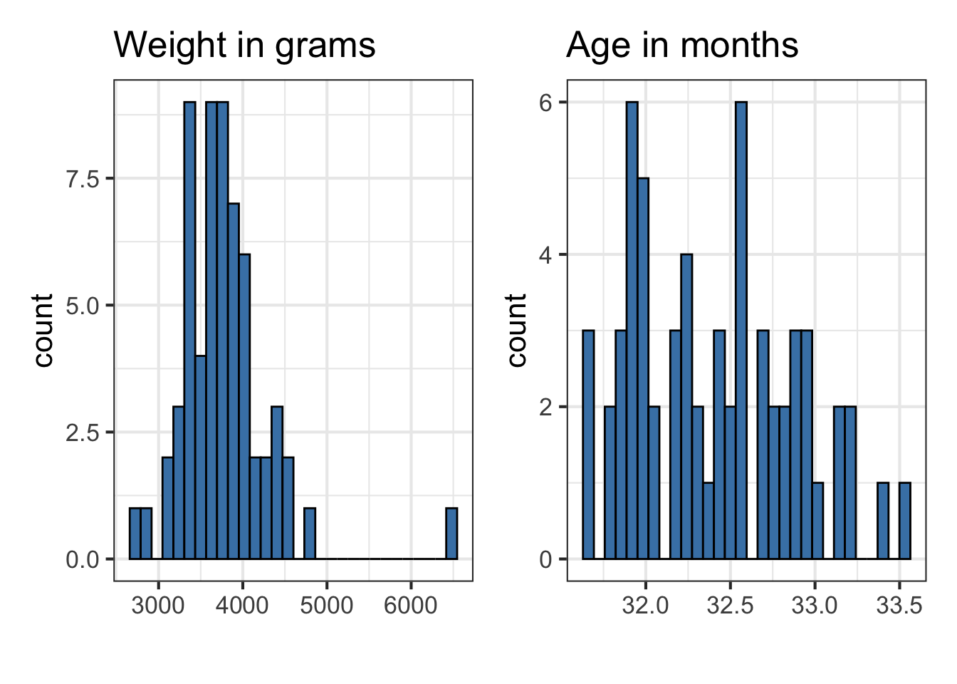
Data: Duke lemurs
Today’s data contains a subset of the original Duke Lemur data set available in the TidyTuesday GitHub repo. This data includes information on “young adult” lemurs from the Coquerel’s sifaka species (PCOQ), the largest species at the Duke Lemur Center. The analysis will focus on the following variables:
age_at_wt_mo: Age in months: Age of the animal when the weight was taken, in months (((Weight_Date-DOB)/365)*12)
weight_g: Weight: Animal weight, in grams. Weights under 500g generally to nearest 0.1-1g; Weights >500g generally to the nearest 1-20g.
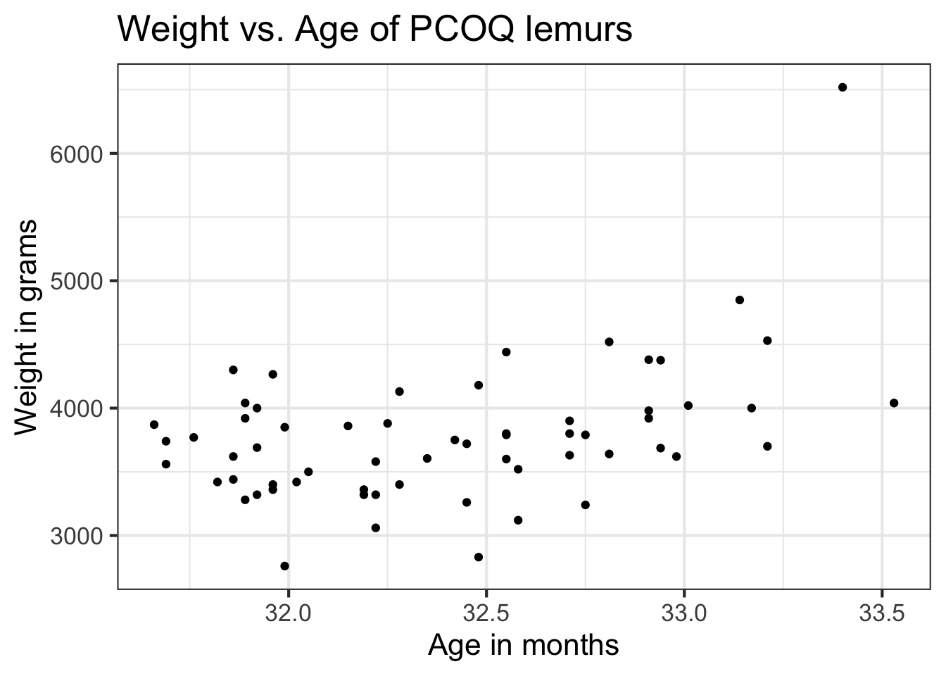
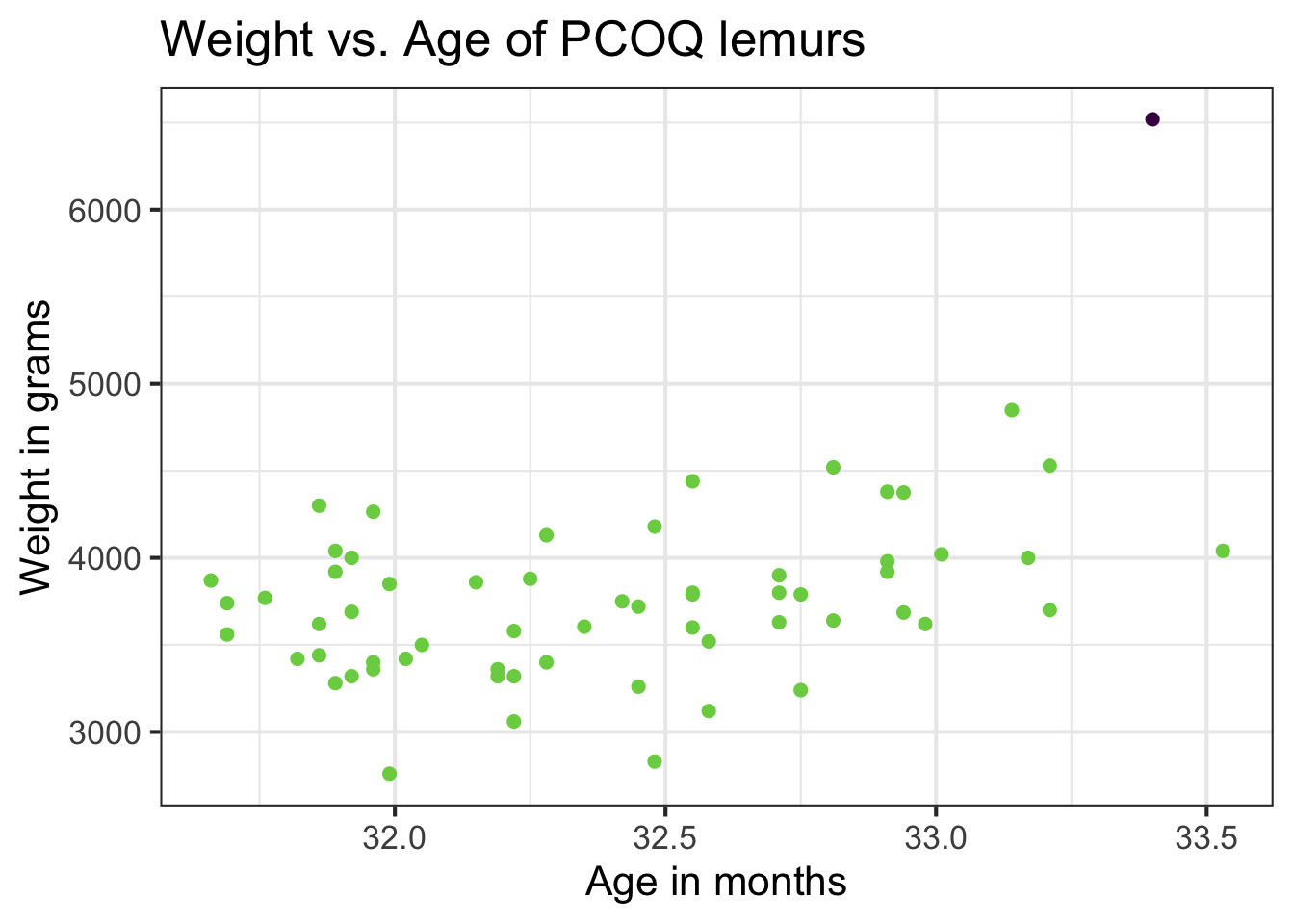
The goal of the analysis is to use the age of the lemurs to understand variability in the weight.
EDA
EDA
Fit model
lemurs_fit <-lm(weight_g ~ age_at_wt_mo, data = lemurs)tidy(lemurs_fit) |>kable(digits =3)
Linearity:\(E[\varepsilon|X] = 0\), i.e. \(E[Y|X] = X\beta\). There is a linear relationship between the response and predictor variables.
Constant variance and independence: \(Var[\varepsilon] = I\sigma^2\). The variability about the least squares line is generally constant and the residuals are independent.
Normality:\(\varepsilon_i \sim Normal\). The distribution of the errors (residuals) is approximately normal.
How do we know if these assumptions hold in our data?
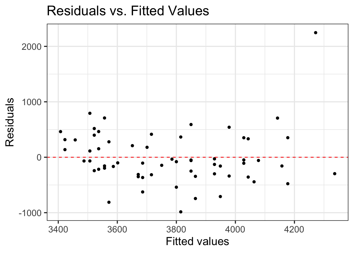
Linearity
Look at plot of residuals versus fitted (predicted) values.
Linearity is satisfied if there is no discernible pattern in the plot (i.e., points randomly scattered around \(residuals = 0\)
Linearity issatisfied
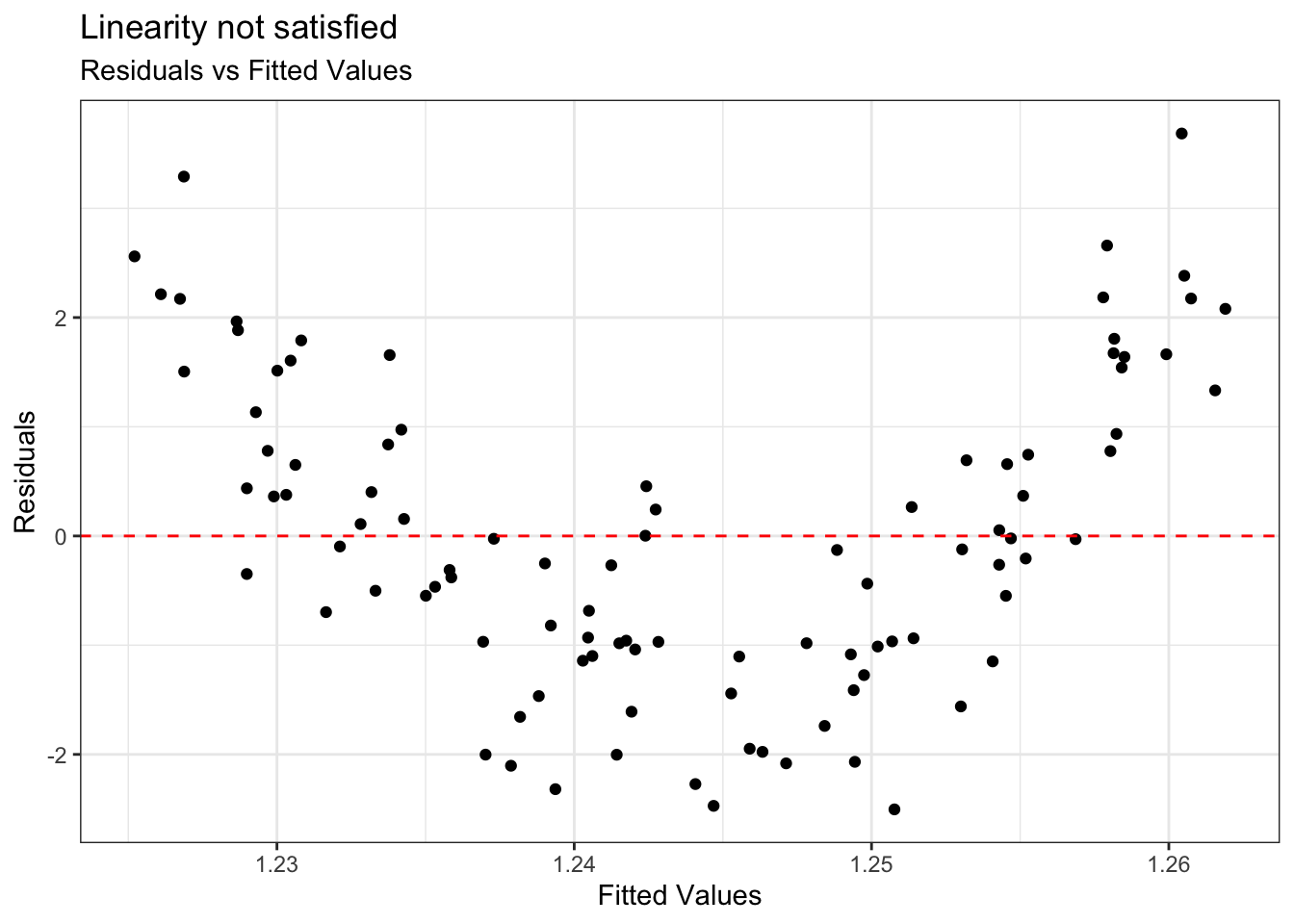
Example: Linearity not satisfied
If linearity is not satisfied, examine the plots of residuals versus each predictor.
Add higher order term(s), as needed.
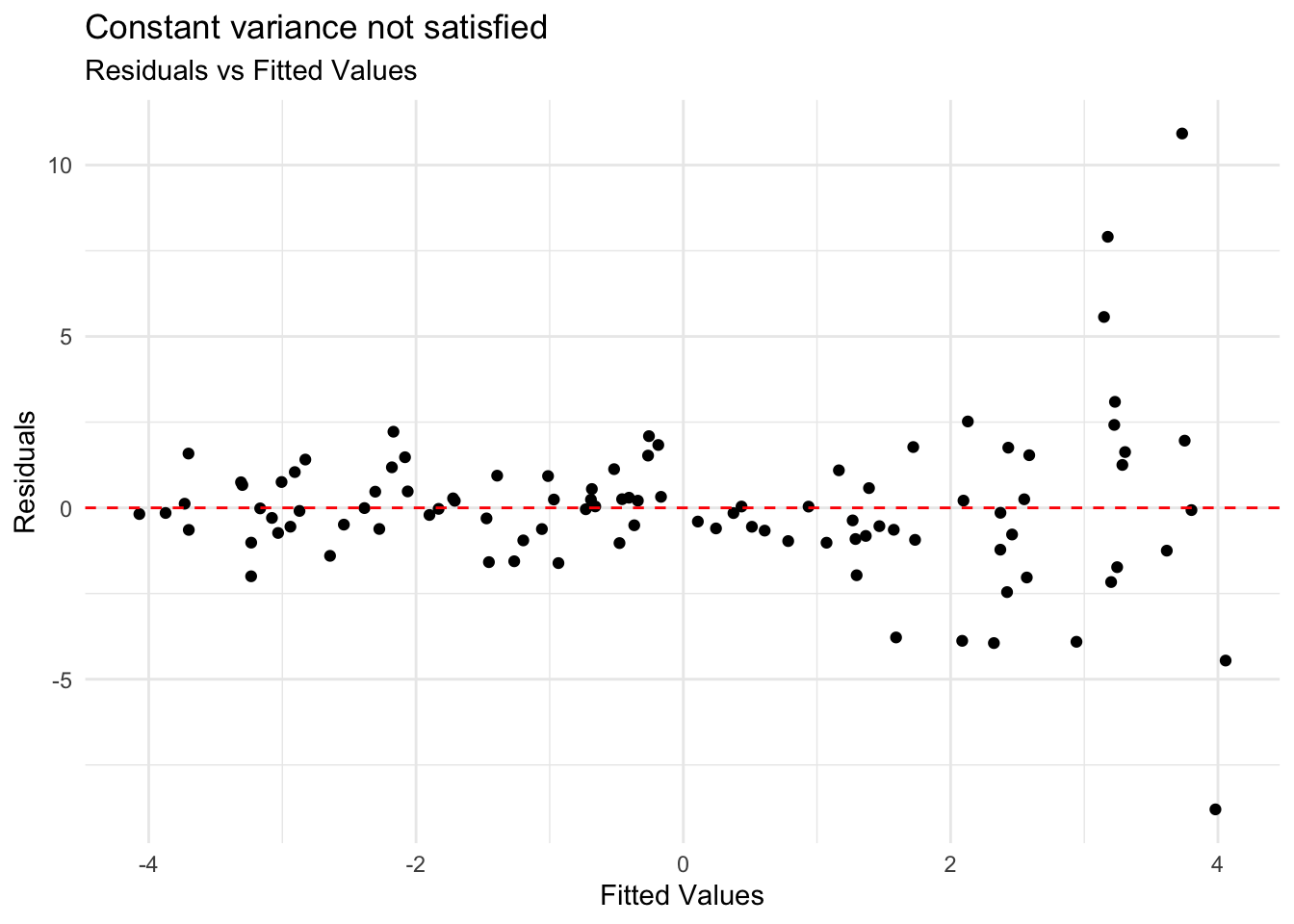
Constant variance
Look at plot of residuals versus fitted (predicted) values.
Constant variance is satisfied if the vertical spread of the points is approximately equal for all fitted values
Constant variance issatisfied
Example: Constant variance not satisfied
Constant variance is critical for reliable inference
Address violations by applying transformation on the response
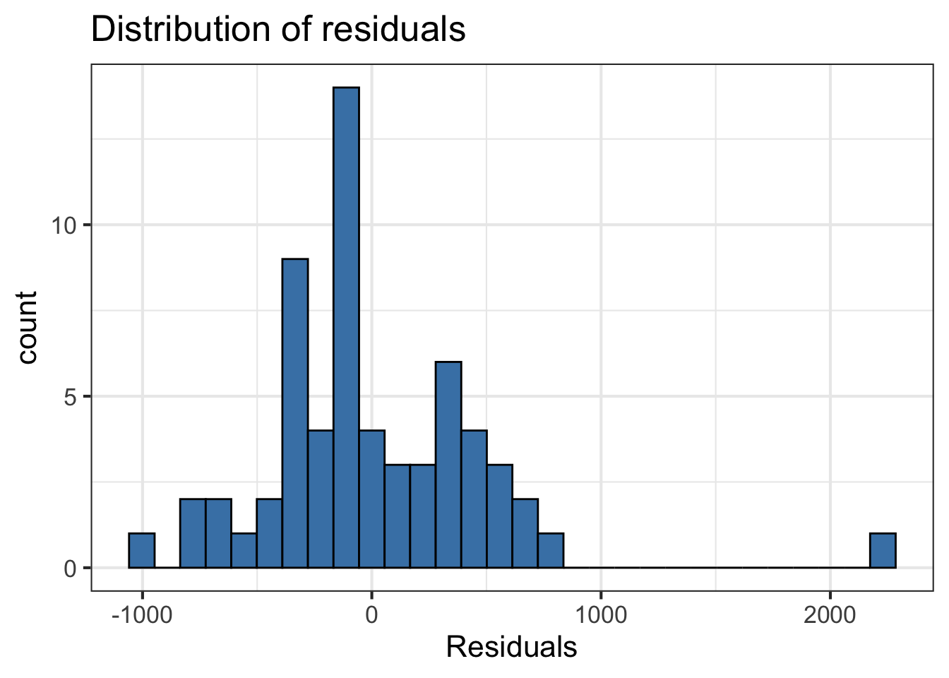
Normality
Look at the distribution of the residuals
Normality is satisfied if the distribution is approximately unimodal and symmetric. Inference robust to violations if \(n > 30\)
`stat_bin()` using `bins = 30`. Pick better value with `binwidth`.
Distribution approximately unimodal and symmetric, aside from the outlier. There are 62 observations, so inference robust to departures.
Independence
We can often check the independence condition based on the context of the data and how the observations were collected.
If the data were collected in a particular order, examine a scatterplot of the residuals versus order in which the data were collected.
If data has spatial element, plot residuals on a map to examine potential spatial correlation.
The independence condition issatisfied. The lemurs could reasonably be treated as independent.
where \(r_i\) is the studentized residual and \(h_{ii}\) is the leverage for the \(i^{th}\) observation
This measure is a combination of
How well the model fits the \(i^{th}\) observation (magnitude of residuals)
How far the \(i^{th}\) observation is from the rest of the data (where the point is in the \(x\) space)
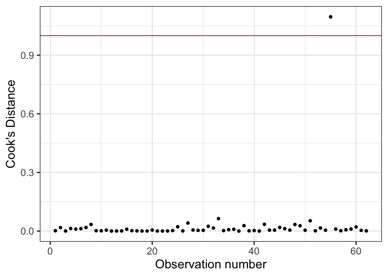
Using Cook’s Distance
An observation with large value of \(D_i\) is said to have a strong influence on the predicted values
General thresholds .An observation with
\(D_i > 0.5\) is moderately influential
\(D_i > 1\) is very influential
Cook’s Distance
Cook’s Distance is in the column .cooksd in the output from the augment() function
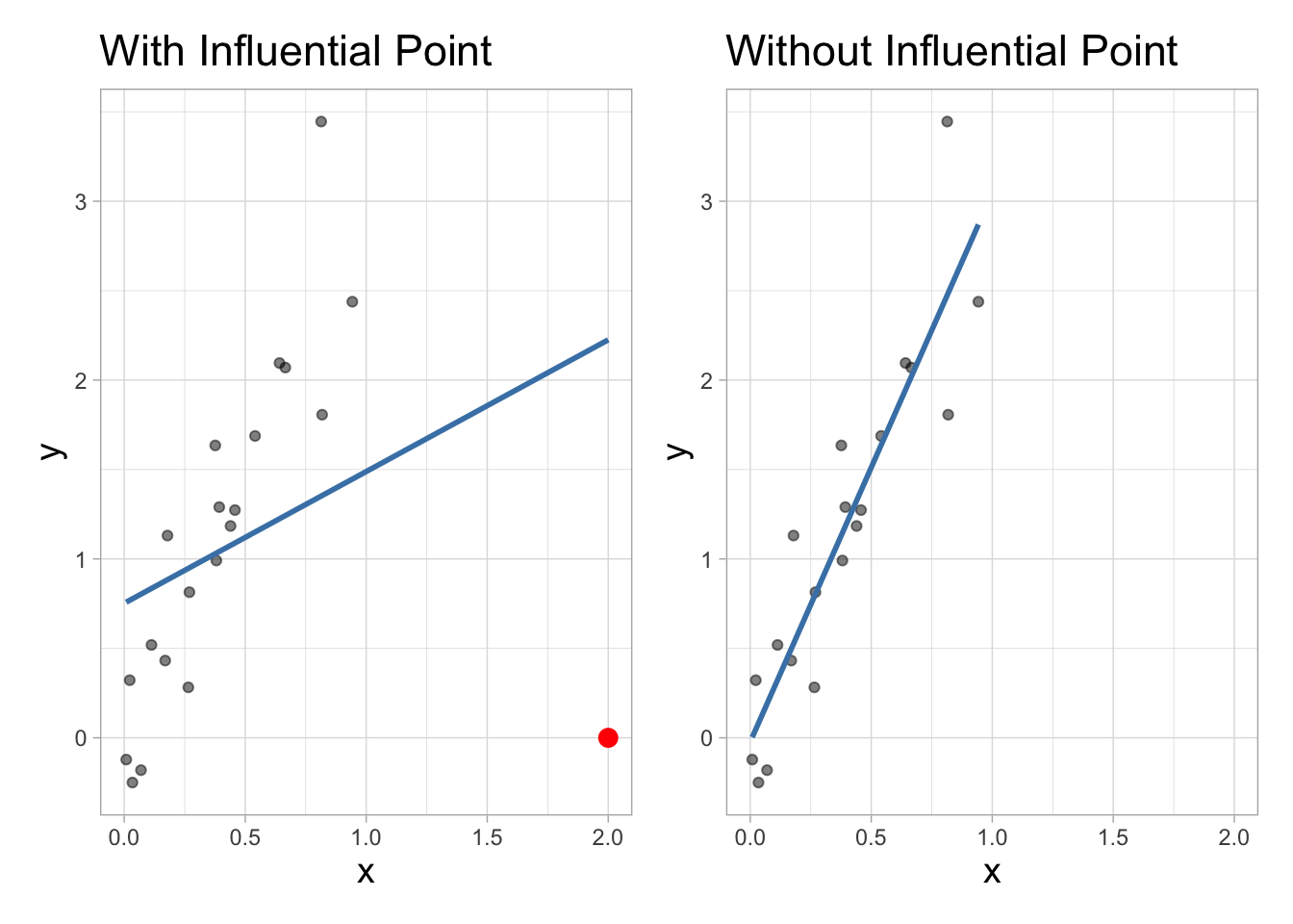
Comparing models
With influential point
term
estimate
std.error
statistic
p.value
(Intercept)
-12314.360
4252.696
-2.896
0.005
age_at_wt_mo
496.591
131.225
3.784
0.000
Without influential point
term
estimate
std.error
statistic
p.value
(Intercept)
-6670.958
3495.136
-1.909
0.061
age_at_wt_mo
321.209
107.904
2.977
0.004
Let’s better understand the influential point.
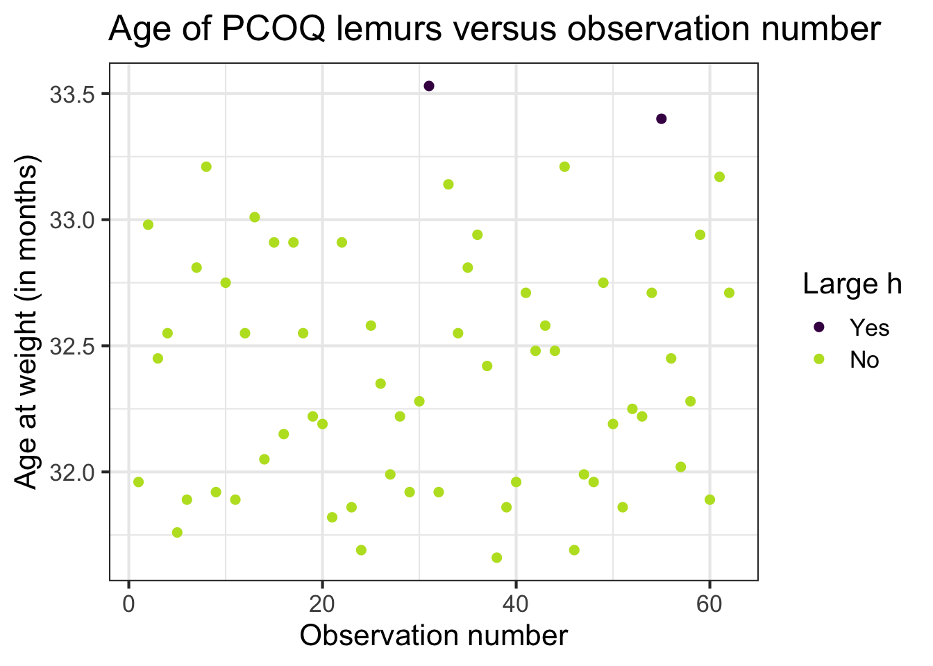
Leverage
Leverage
Recall the hat matrix\(\mathbf{H} = \mathbf{X}(\mathbf{X}^\mathsf{T}\mathbf{X})^{-1}\mathbf{X}^\mathsf{T}\)
We focus on the diagonal elements
\[
h_{ii} = \mathbf{x}_i^\mathsf{T}(\mathbf{X}^\mathsf{T}\mathbf{X})^{-1}\mathbf{x}_i
\]such that \(\mathbf{x}^\mathsf{T}_i\) is the \(i^{th}\) row of \(\mathbf{X}\)
\(h_{ii}\) is the leverage: a measure of the distance of the \(i^{th}\) observation from the center (or centroid) of the \(x\) space
Observations with large values of \(h_{ii}\) are far away from the typical value (or combination of values) of the predictors in the data
Large leverage
The sum of the leverages for all points is \(p\), where \(p\) is the number of predictors (+ intercept) in the model . More specifically
\[
\sum_{i=1}^n h_{ii} = \text{rank}(\mathbf{H}) = \text{rank}(\mathbf{X}) = p
\]
The average value of leverage, \(h_{ii}\), is \(\bar{h} = \frac{(p)}{n}\)
An observation has large leverage if \[h_{ii} > \frac{2(p)}{n}\]
Why do you think these points have large leverage?
Let’s look at the data
Large leverage
If there is point with high leverage, ask
Is there a data entry error?
Is this observation within the scope of individuals for which you want to make predictions and draw conclusions?
Is this observation impacting the estimates of the model coefficients? (Need more information!)
Just because a point has high leverage does not necessarily mean it will have a substantial impact on the regression. Therefore we need to check other measures.
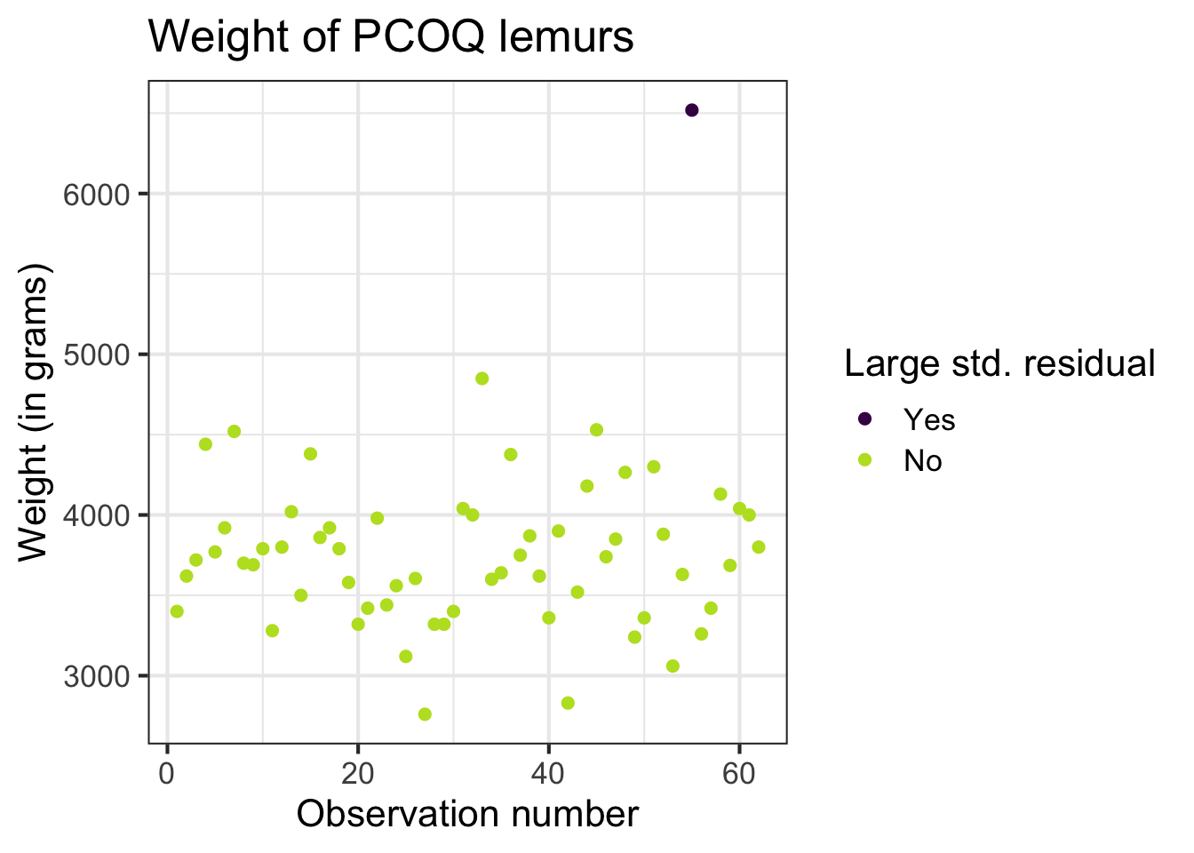
Scaled residuals
Scaled residuals
What is the best way to identify outlier points that don’t fit the pattern from the regression line?
Look for points that have large residuals
We can rescale residuals and put them on a common scale to more easily identify “large” residuals
We will consider two types of scaled residuals: standardized residuals and studentized residuals
Standardized residuals
The variance of the residuals can be estimated by the mean squared residuals (MSR) \(= \frac{SSR}{n - p} = \hat{\sigma}^2_{\varepsilon}\)
Standardized and studentized residuals provide similar information about which points are outliers in the response.
Studentized residuals are used to compute Cook’s Distance.
Using these measures
Standardized residuals, leverage, and Cook’s Distance should all be examined together
Examine plots of the measures to identify observations that are outliers, high leverage, and may potentially impact the model.
Back to the influential point
What to do with outliers/influential points?
First consider if the outlier is a result of a data entry error.
If not, you may consider dropping an observation if it’s an outlier in the predictor variables if…
It is meaningful to drop the observation given the context of the problem
You intended to build a model on a smaller range of the predictor variables. Mention this in the write up of the results and be careful to avoid extrapolation when making predictions
What to do with outliers/influential points?
It is generally not good practice to drop observations that are outliers in the value of the response variable
These are legitimate observations and should be in the model
You can try transformations or increasing the sample size by collecting more data
A general strategy when there are influential points is to fit the model with and without the influential points and compare the outcomes