View libraries and data sets used in these notes
library(tidyverse)
library(tidymodels)library(tidyverse)
library(tidymodels)\[ X \sim N(\mu, \sigma^2) \]
We read the above mathematical statement: “the random variable X is normally distributed with mean mu and variance sigma-squared.”
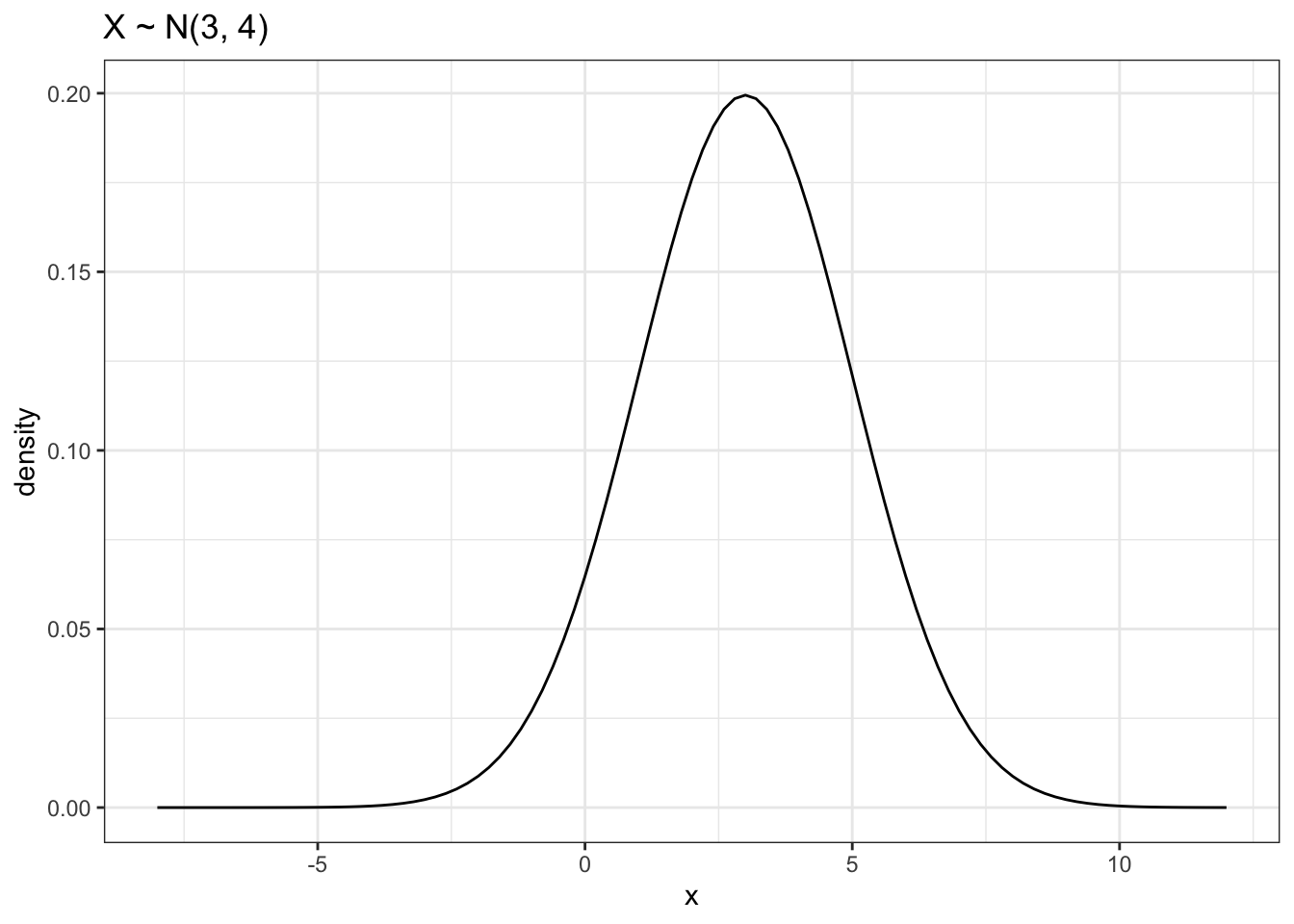
data.frame(x = -8:12) |>
  ggplot(aes(x = x)) +
  stat_function(fun = dnorm, args = list(mean = 3, sd = 2)) +
  theme_bw() +
labs(title = "X ~ N(3, 4)", y = "density")The normal distribution, also known as “Gaussian distribution” is a distribution of a continuous random variable. The sample space of a normal random variable is \(\{- \infty, + \infty \}\) and is defined by two parameters: a mean \(\mu\) and a standard deviation \(\sigma\). The mean is known as the location parameter while the standard deviation is the scale.
We can sample N times from a normal with mean mu and standard deviation sigma using rnorm(n = N, mean = mu, sd = sigma).
rnorm(n = 1000, mean = 10, sd = 1) |>
  hist()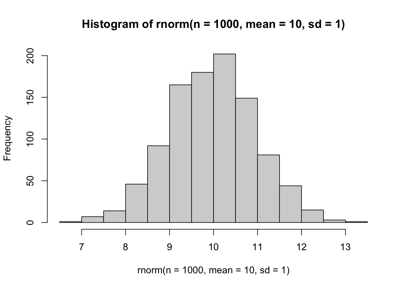
A very useful property of Normal distribution is that it is stable. What this means is that linear combinations of normal random variables are themselves normal. In other words, if \(X\) and \(Y\) are normal random variables then \(aX + bY\) is normal for all \(a\) and \(b\). The two properties to remember when adding Gaussian random variables are:
We can see this in an example.
Let \(X \sim N(5, 9)\) and let \(Y \sim N(-5, 1)\)
According to our rules above \(X + Y \sim N(0, 10)\). Let’s check ourselves with code:
set.seed(1)
normal_df = data.frame(X = rnorm(1000, mean = 5, sd = 3),
                 Y = rnorm(1000, mean = -5, sd = 1))


normal_df = normal_df %>%
  mutate(Z = X + Y)

normal_df %>%
  ggplot(aes(x = Z)) +
  geom_histogram(aes(y = ..density..), fill = 'gold3', alpha = 0.5) +
  theme_bw() +
  labs(y = "Density", title = "Matching densities") +
  stat_function(fun = dnorm, args = list(mean = 0, sd = sqrt(10)),
                color = "darkblue")
Let \(Z \sim N(0, 1)\) and \(X \sim N(10, 16)\). \(aZ + b \stackrel{d}{=} X\) for some \(a\) and \(b\). What are \(a\) and \(b\)? Fill them in for the ? in the code below and the uncomment the code. Here, \(\stackrel{d}{=}\) means “equal in distribution”.
set.seed(221)
normal_df = data.frame(z = rnorm(1000, mean = 0, sd = 1),
                 x = rnorm(1000, mean = 10, sd = 4))

sample_mean = normal_df %>%
  summarize(sample_mean = mean(x)) %>%
  pull()

normal_df %>%
  ggplot(aes(x = x)) +
  geom_histogram(aes(y = ..density..), fill = 'gold3', alpha = 0.5) +
  geom_histogram(aes(x = z, y = ..density..), fill = 'steelblue', alpha = 0.7) +
  #geom_density(aes(x = z*? + ?), color = 'red') +
  theme_bw() +
  labs(x = "", y = "", title = "Sampling from two normals")
Another useful property is that the marginal distribution of a multivariate normal itself normal.
Let \[ \begin{bmatrix} X \\ Y \end{bmatrix} \sim MVN\left( \begin{bmatrix} \mu_X \\ \mu_Y \end{bmatrix}, \; \begin{bmatrix} \sigma_X^2 & \sigma_{XY} \\ \sigma_{XY} & \sigma_Y^2 \end{bmatrix} \right). \]
Then the marginal distributions are \[ X \sim N(\mu_X, \sigma_X^2), \qquad Y \sim N(\mu_Y, \sigma_Y^2). \]
Note: if you’d like to simulate from a multivariate normal, you can use the function rmvnorm() from the mvtnorm package.
mvtnorm::rmvnorm(n = 3, mean = c(0, 10), sigma =
                   matrix(c(2, .5, .5, 1), ncol = 2))
[,1] [,2]
[1,] -1.64375527 7.934314
[2,] 2.37437357 10.848478
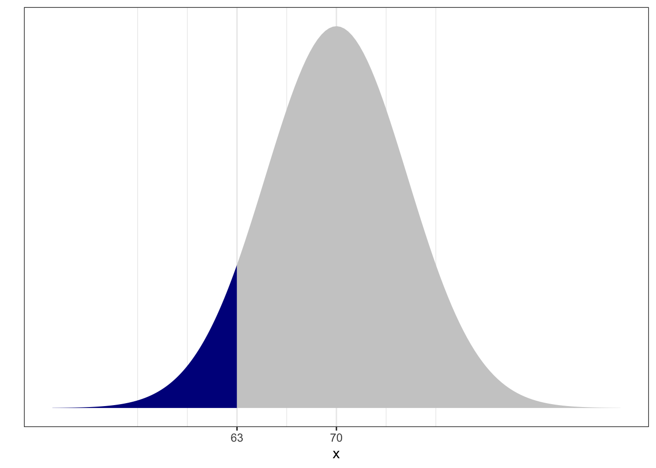
[3,] 0.06844319 10.669071pnorm “probability normal” takes three arguments:
q, mean and sdand pnorm(q = q, mean = mu, sd = sigma) answers the question:
If \(X \sim N(\mu, \sigma)\), what is \(p(X < q)\)?
For example, imagine that the resting heart rates in the classroom are normally distributed with mean 70 beats per minute (bpm) and standard deviation 5 bpm. What’s the probability a randomly selected individual has a heart rate less than 63 bpm?
In math: let \(X\) be the bpm of an individual in this class. Assume \(X \sim N(70, 25)\). What is \(p(X < 63)\)? Given heartbeats are normally distributed, randomly selecting an individual from the classroom is called “drawing from a normal distribution”.
We can compute this easily:
pnorm(63, mean = 70, sd = 5)[1] 0.080756660.08 or about 8% chance. In picture, the probability is the proportion of area under the curve shaded:
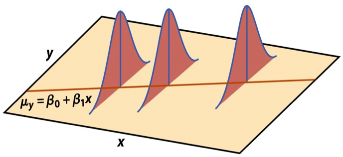
Recall the main question we had before: what assumptions make \(\hat{\beta}_{OLS}\) representative of \(\beta\)?
Taken all together, we can write assumptions 1, 2, and 3 concisely:
\[ \boldsymbol{\varepsilon}\sim MVN(\boldsymbol{0}, \sigma^2 \boldsymbol{I}) \] or equivalently,
\[ \varepsilon_i \stackrel{\text{i.i.d.}}{\sim} \; N(0, \sigma^2) \text{ for each i} \]
The implications of this assumption are:
\[ \boldsymbol{y}\sim MVN_n(\boldsymbol{X}\beta, \sigma^2 \boldsymbol{I}) \]
or equivalently,
\[ y_i \sim N(x_i^T \beta, \sigma^2). \]
Moreover,
\[ \hat{\beta} \sim MVN(\beta, \sigma^2 (\boldsymbol{X}^T\boldsymbol{X})^{-1}) \] which implies that the marginal distribution of a single element of the \(\hat{\beta}\),
\[ \hat{\beta}_j \sim N(\beta_j, \sigma^2 C_{jj}) \] where the matrix \(C = (\boldsymbol{X}^T\boldsymbol{X})^{-1}\) and \(C_{jj}\) is the \(j\)th diagonal element.
Based on the properties of a normal described above,
\[ \frac{\hat{\beta}_j - \beta_j}{\sqrt{\sigma^2 C_{jj}}} \sim N(0, 1) \]
Where this is going: checking our assumptions are valid, constructing confidence intervals, and performing hypothesis tests.
An important view of the equation above,
\[ y_i \sim N(x_i^T \beta, \sigma^2), \] is that it can be used to generate data. For this reason, the statistical model is often called a “data generative model”.
It looks like this:
create length n vector \(x\). For example, x <- runif(n, 0, 10)
specify the true \(\beta\), e.g. beta0 <- 1; beta1 <- 2
choose some error \(\sigma^2\) and generate \(y_i\) according to the data generative model: rnorm(n, mean = (beta0 + beta1 * x, sd = 2)).
From here you can fit the data with lm(y ~ x) and examine the results.