Introduction to inference

library(tidyverse)
library(tidymodels)
library(DT)
library(latex2exp)
library(patchwork)

pokemon <- read_csv("https://sta221-fa25.github.io/data/pokemon_data.csv") # complete, population data

The data

As of 2025, there are 1025 pokemon in existence.

In all statistical inference tasks, we only have a sample from the population. Let’s consider a random sample of the pokemon data, given below:

set.seed(48) 
pokemon_sample <- pokemon |>
  slice_sample(n = 15) |>
  select(dexnum, name, height_m, weight_kg) |>
  arrange(dexnum)
  

datatable(pokemon_sample, rownames = FALSE, options = list(pageLength = 5),
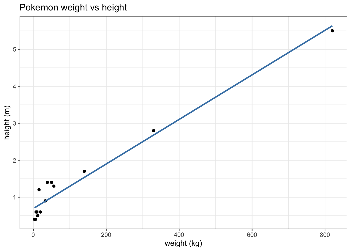
           caption = "sample of 15 pokemon")

Let’s investigate the question: are heavier pokemon taller?

plot

linear model

lm(height_m ~ weight_kg, data = pokemon_sample) |>
  tidy()

# A tibble: 2 × 5
  term        estimate std.error statistic  p.value
  <chr>          <dbl>     <dbl>     <dbl>    <dbl>
1 (Intercept)  0.692    0.0859        8.06 2.07e- 6
2 weight_kg    0.00603  0.000369     16.3  4.90e-10

plot code

pokemon_sample |>
  ggplot(aes(x = weight_kg, y = height_m)) +
  geom_point() +
  geom_smooth(method = 'lm', se = FALSE, color = 'steelblue') +
  theme_bw() +
  labs(title = "Pokemon weight vs height", y = "height (m)", x = "weight (kg)")

Question

How can we tell if our estimates \(\hat{\beta}\) are any good?

repeated sampling

pokemon_hw = pokemon |>
  select(height_m, weight_kg)

BETA_HAT <- NULL
for(i in 1:1000) {
  fit <- pokemon_hw |>
    slice_sample(n = 15) |> 
    lm(height_m ~ weight_kg, data = _) 
  BETA_HAT <- rbind(BETA_HAT, fit$coefficients)
}

BETA_HAT <- data.frame(BETA_HAT)
colnames(BETA_HAT) <- c("beta0", "beta1")

glimpse(BETA_HAT)

Rows: 1,000
Columns: 2
$ beta0 <dbl> 0.9016025, 0.5209848, 0.6775509, 0.8639395, 0.4678607, 0.4351285…
$ beta1 <dbl> 0.004823824, 0.010159875, 0.008377374, 0.012071556, 0.016425420,…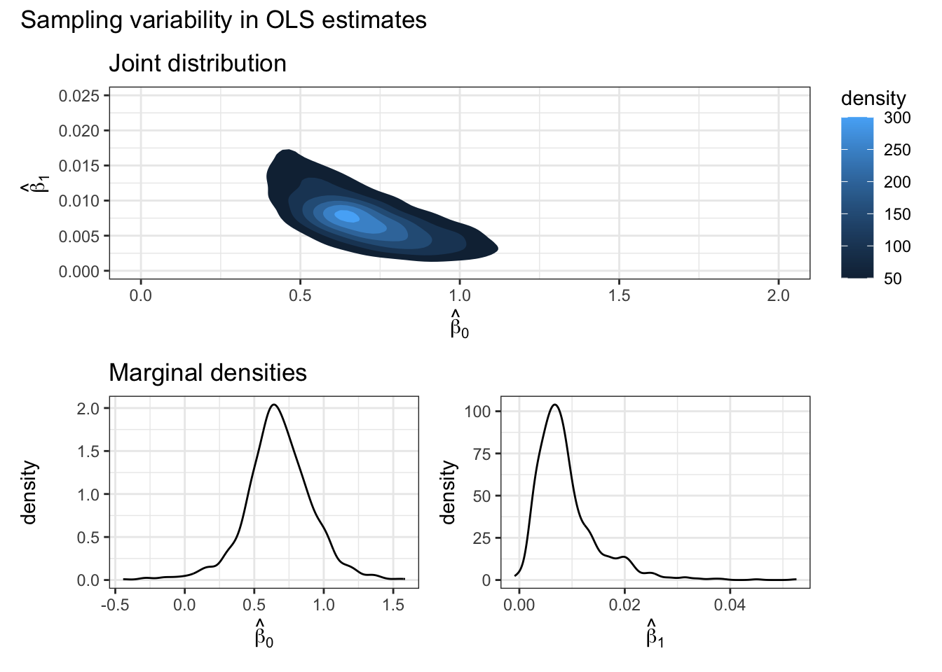

plots

population-level annotation

popn_model <- lm(height_m ~ weight_kg, data = pokemon)
popn_model$coefficients

(Intercept)   weight_kg 
0.775612595 0.006509202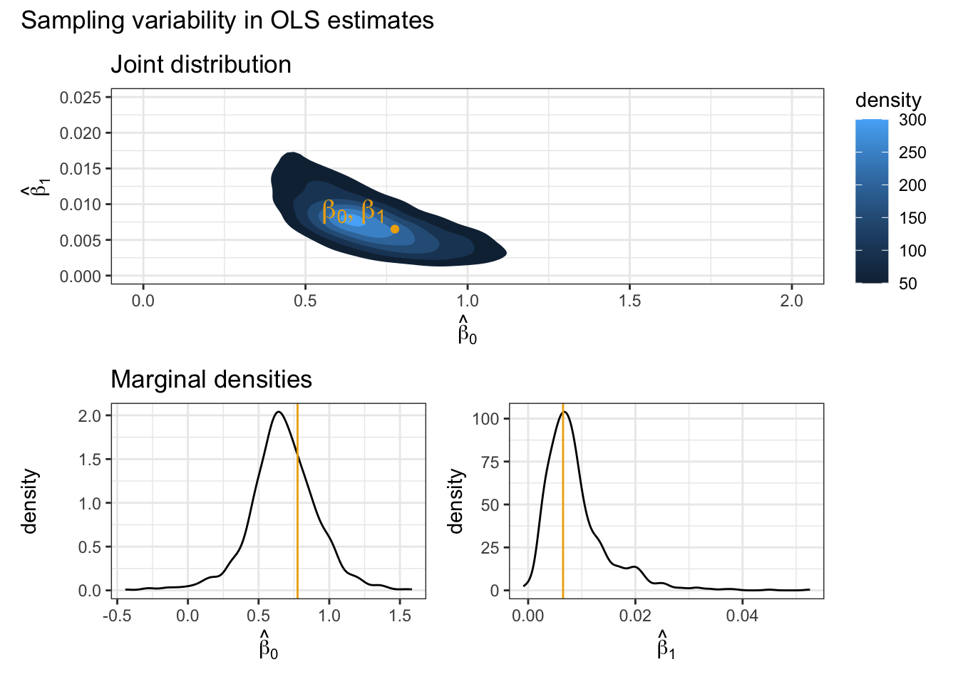 

Framework

Our objective is to infer properties about a population using data from an experiment or survey (in this case, a survey/sample of pokemon).

Post-experiment: after collecting the data, \(\hat{\beta}_0, \hat{\beta}_1\) are fixed and known.

Pre-experiment: before collecting the data, the data are unknown and random. \(\hat{\beta}_0, \hat{\beta}_1\), which are functions of the data, are also unknown and random.

In all cases, the true population parameters, \(\beta_0, \beta_1\) are fixed but unknown.

Pre-experimental question: is the probability distribution of \(\hat{\beta}_0, \hat{\beta}_1\) a meaningful representation of the population?

Answer: this depends on certain assumptions we make about population.

Assumption 1

\(E[\boldsymbol{\varepsilon}|\boldsymbol{x}] = \boldsymbol{0}\), or equivalently, \(E[\varepsilon_i|\boldsymbol{x}] = 0\) for all \(i\).

Implications: in simple linear regression, assumption 1 implies that \(E[y_i|\boldsymbol{x}] = E[\beta_0 + \beta_1 x_i + \epsilon_i|\boldsymbol{x}] = E[\beta_0 |\boldsymbol{x}] + E[\beta_1 x_i|\boldsymbol{x}] + E[\epsilon_i|\boldsymbol{x}] = \beta_0 + \beta_1 x_i\).

Exercise

Show that assumption 1 implies that \(E[\hat{\beta}|\boldsymbol{X}] = \beta\).

Solution

\[ \begin{aligned} E[\hat{\beta}|\boldsymbol{X}] &= E[(\boldsymbol{X}^T\boldsymbol{X})^{-1}\boldsymbol{X}^T\boldsymbol{y}| \boldsymbol{X}]\\ &= (\boldsymbol{X}^T\boldsymbol{X})^{-1}\boldsymbol{X}^T E[\boldsymbol{y}| \boldsymbol{X}]\\ &= (\boldsymbol{X}^T\boldsymbol{X})^{-1}\boldsymbol{X}^T \boldsymbol{X}\beta\\ &= \beta \end{aligned} \]

Since \(E[\hat{\beta}|\boldsymbol{X}] = \beta\), we say \(\hat{\beta}\) is an unbiased estimator of \(\beta\).

Notice that this result (unbiasedness) does not depend independence of errors, normality, or constant variance.

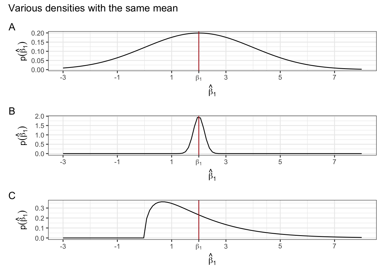
However, the result doesn’t tell us anything about how close \(\hat{\beta}\) will be to \(\beta\). The estimator may be unbiased, but by itself, this doesn’t tell us much. See examples of “unbiased” distributions of an estimator below.