Model assessment

Author

Dr. Alexander Fisher

View libraries and data sets used in these notes

library(tidyverse) # data wrangling and visualization
library(DT) # shows the data table
library(patchwork) # arranging plots
library(tidymodels)  # modeling (includes broom, yardstick, and other packages)
library(knitr)       # aesthetic tables
 
life_exp <- read_csv(
    "https://sta221-fa25.github.io/data/life-expectancy-data.csv") |> 
  rename(life_exp = `Life_expectancy_at_birth`, 
         income_inequality = `Income_inequality_Gini_coefficient`) |>
  mutate(education = if_else(Education_Index > median(Education_Index), "High", "Low"), 
         education = factor(education, levels = c("Low", "High"))) |>
  select(Country, life_exp, Health_expenditure, income_inequality)

Learning objectives

By the end of today you will be able to

fit simple linear regression models in R
interpret coefficients in context
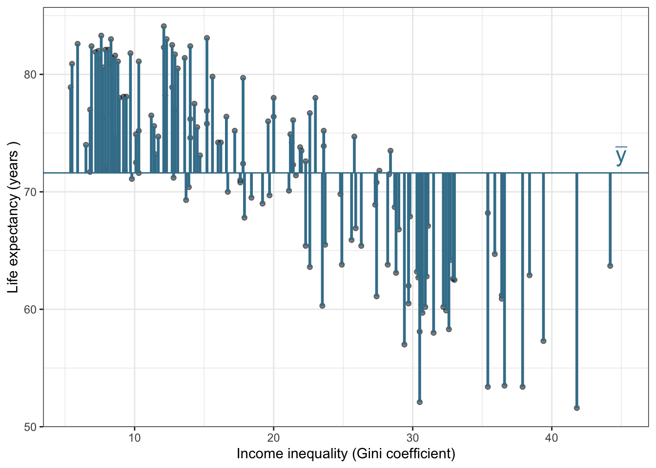
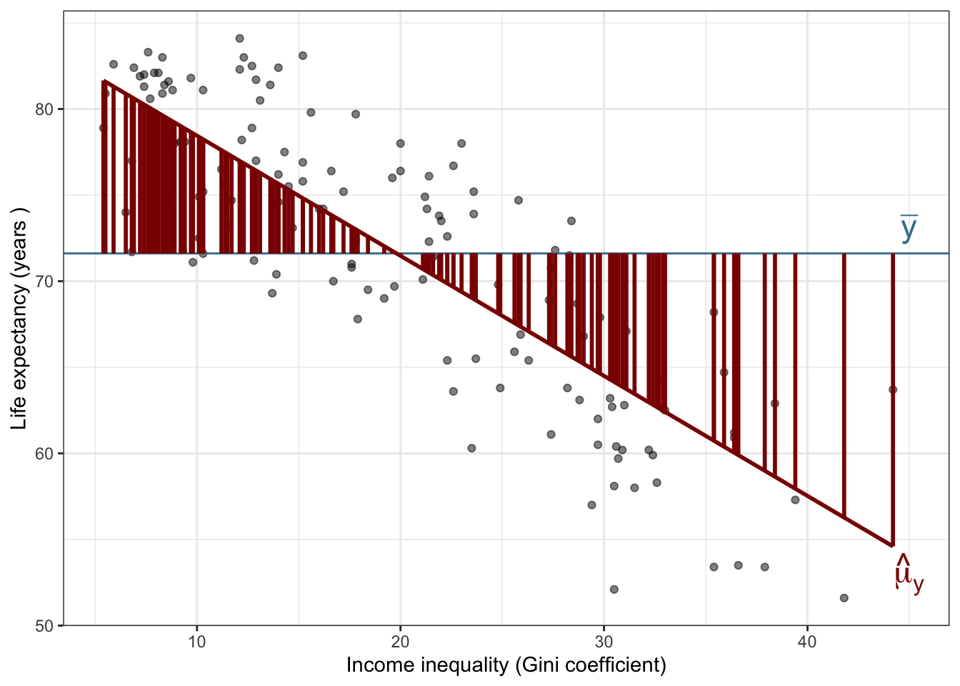
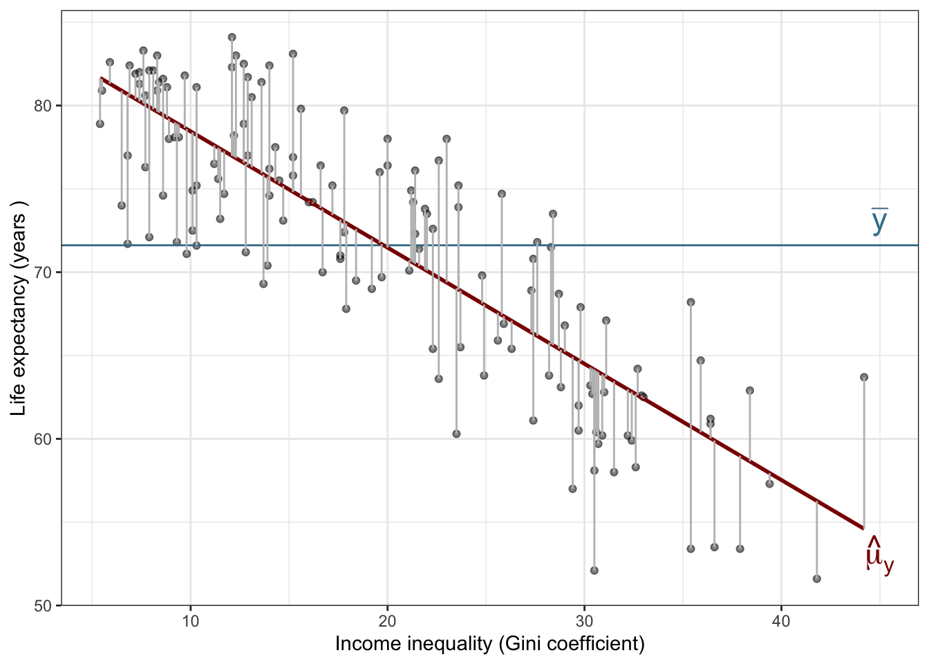
analyze the variance
check model fit and interpret in context

Example

The data set comes from Zarulli et al. (2021) who analyze the effects of a country’s healthcare expenditures and other factors on the country’s life expectancy. The data are originally from the Human Development Database and World Health Organization.

There are 140 countries (observations) in the data set.

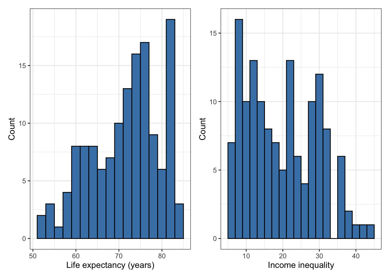
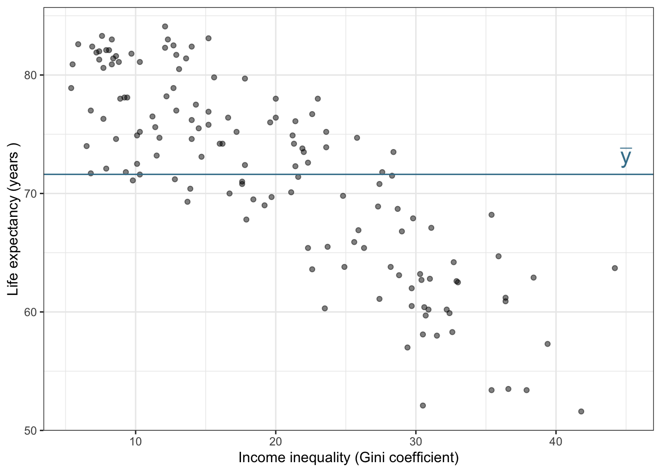
Goal: Use the income inequality in a country to understand variability in the life expectancy.

Click here for the original research paper.

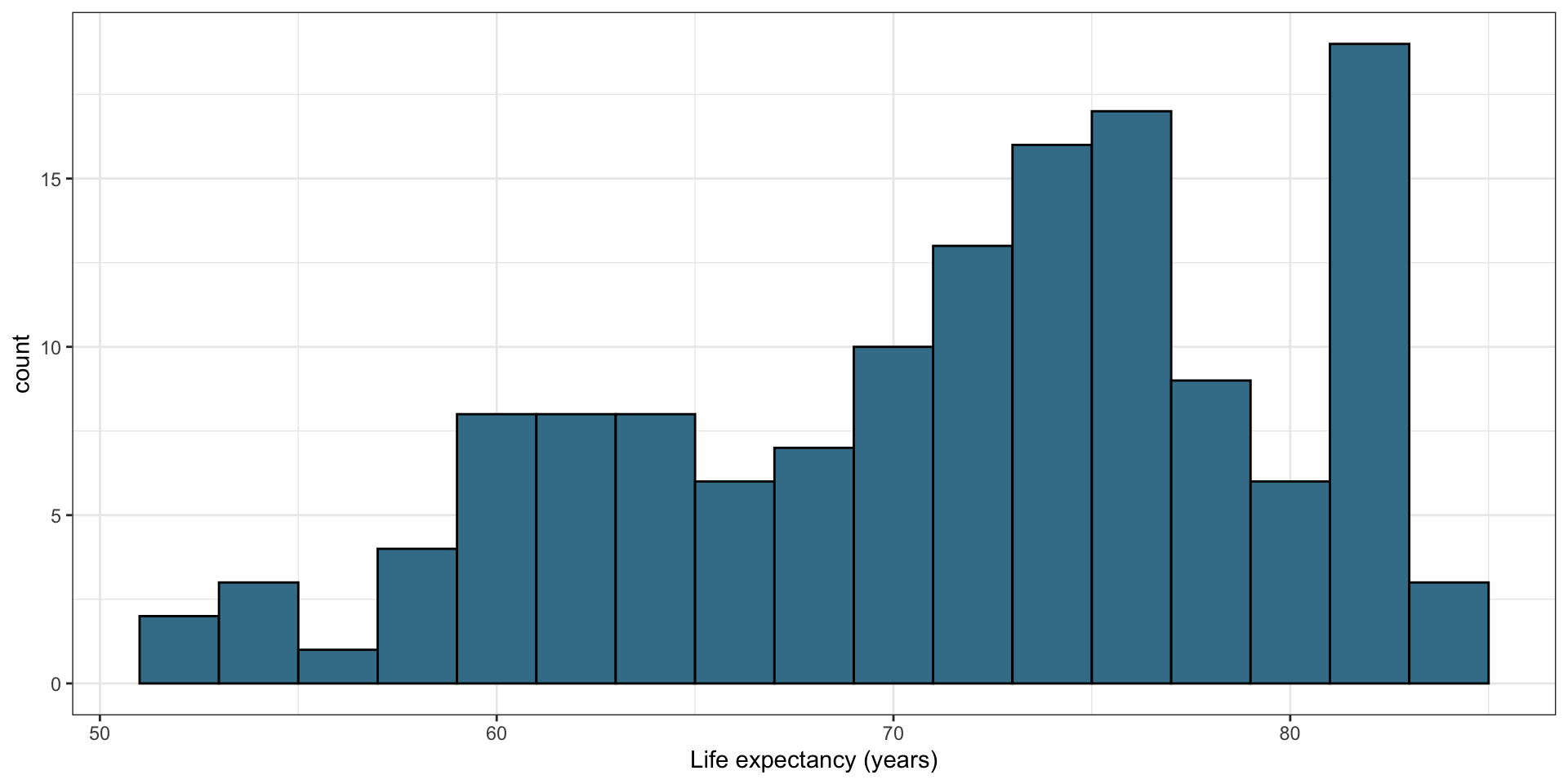
life_exp: The average number of years that a newborn could expect to live, if he or she were to pass through life exposed to the sex- and age-specific death rates prevailing at the time of his or her birth, for a specific year, in a given country, territory, or geographic area (from the World Health Organization).
income_inequality: Measure of the deviation of the distribution of income among individuals or households within a country from a perfectly equal distribution. A value of 0 represents absolute equality, a value of 100 absolute inequality, based on “Gini coefficient” (from Zarulli et al. (2021)).
health_expenditure: Per capita current spending on healthcare goods and services, expressed in respective currency - international Purchasing Power Parity (PPP) dollar (from the World Health Organization)

Exploratory data analysis (EDA)

p1 <- ggplot(data = life_exp, aes(x = life_exp))  + 
  geom_histogram(fill = "steelblue", color = "black", binwidth = 2) + 
  labs(x = "Life expectancy (years)", 
       y = "Count") +
  theme_bw()

p2 <- ggplot(data = life_exp, aes(x = income_inequality))  + 
  geom_histogram(fill = "steelblue", color = "black", binwidth = 2) + 
  labs(x = "Income inequality", 
       y = "Count") +
  theme_bw()

p1 + p2 # uses patchwork package

Bivariate EDA

plot
code

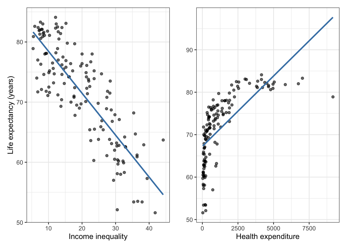
# Scatterplot of life expectancy vs income inequality
p1 <- ggplot(life_exp, aes(x = income_inequality, y = life_exp)) +
  geom_point(alpha = 0.6) +
  geom_smooth(method = "lm", se = FALSE, color = "steelblue") +
  labs(
    x = "Income inequality",
    y = "Life expectancy (years)"
  ) +
  theme_bw()

# Scatterplot of life expectancy vs health expenditure
p2 <- ggplot(life_exp, aes(x = Health_expenditure, y = life_exp)) +
  geom_point(alpha = 0.6) +
  geom_smooth(method = "lm", se = FALSE, color = "steelblue") +
  labs(
    x = "Health expenditure",
    y = ""
  ) +
  theme_bw()

# Display plots side by side; uses patchwork pacakge
p1 + p2

Ordinary least squares regression in R

Template

To fit a model by OLS linear regression, we use the lm function. The arguments look as follows:

lm(y ~ x, data = data_frame)

In words, we “regress y on x” where “y” and “x” are column names in the data frame “data_frame”.

For our data

# income inequality model
model_ii = lm(life_exp ~ income_inequality, 
              data = life_exp)

# health expenditure model
model_he = lm(life_exp ~ Health_expenditure,
              data = life_exp)

Q: why is Health_expenditure capitalized, but income_inequality is not?
A: That’s how they are named in the data! See the column names: names(life_exp).

Look at results (income inequality model)

Regular output:

model_ii


Call:
lm(formula = life_exp ~ income_inequality, data = life_exp)

Coefficients:
      (Intercept)  income_inequality  
          85.4202            -0.6973

Tidy the output:

model_ii |>
  tidy()

# A tibble: 2 × 5
  term              estimate std.error statistic   p.value
  <chr>                <dbl>     <dbl>     <dbl>     <dbl>
1 (Intercept)         85.4      0.855       99.9 1.41e-130
2 income_inequality   -0.697    0.0388     -18.0 6.17e- 38

Put results in a more aesthetic table using kable from the knitr package:

model_ii |>
  tidy() |> 
  kable(digits = 3)

term	estimate	std.error	statistic	p.value
(Intercept)	85.420	0.855	99.877	0
income_inequality	-0.697	0.039	-17.961	0

The fitted regression model:

\[ \hat{y_i} = 85.420 - 0.697 x_i \]

Interpretation

The intercept estimate \(\hat{\beta}_0\) is in units of the response variable. It is the expected value of the response variable when the predictor is set to 0.
The estimate of the slope coefficient, \(\hat{\beta}_1\) is measured in the units of the response variable per unit of the explanatory variable.

Exercise

Interpret the coefficients above (for the income inequality model) in context.

Prediction

Use the predict function to calculate predictions for new observations

Single observation

new_ii <- tibble(income_inequality = 50)
predict(model_ii, new_ii)

       1 
50.55618

Multiple observations

more_new_ii <- tibble(income_inequality = c(25,50, 100))
predict(model_ii, more_new_ii)

       1        2        3 
67.98821 50.55618 15.69213

Note the range:

range(life_exp$income_inequality)

[1]  5.4 44.2

Caution

Using the model to predict for values outside the range of the original data is extrapolation. Why do we want to avoid extrapolation?

Model assessment

We fit a model but is it any good?

Two statistics

Root mean square error, RMSE: A measure of the average error (average difference between observed and predicted values of the outcome)
R-squared, \(R^2\) : Percentage of variability in the outcome explained by the regression model (in the context of SLR, the predictor)

What indicates a good model fit? Higher or lower RMSE? Higher or lower \(R^2\)?

RMSE

\[ RMSE = \sqrt{\frac{\sum_{i=1}^n(y_i - \hat{y}_i)^2}{n}} = \sqrt{\frac{\sum_{i=1}^ne_i^2}{n}} \]

ANOVA and \(R^2\)

ANOVA

Analysis of Variance (ANOVA): Technique to partition variability in \(Y\) by the sources of variability

Total variability (Response)

Min	Median	Max	Mean	Std.Dev
51.6	72.85	84.1	71.614	8.075

Partition sources of variability in `life_exp`

Total variability (Response)

\[\text{Sum of Squares Total (SST)} = S_{yy} = \sum_{i=1}^n(y_i - \bar{y})^2 = (n-1) \cdot var(y)\]

Explained variability (Model)

\[\text{Sum of Squares Model (SSM)} = \sum_{i = 1}^{n}(\hat{y}_i - \bar{y})^2\]

Unexplained variability (Residuals)

\[\text{Sum of Squares Residuals (SSR)} = \sum_{i = 1}^{n}(y_i - \hat{y}_i)^2\]

Sum of Squares

\[ \begin{aligned} \color{#407E99}{SST} \hspace{5mm}&= &\color{darkred}{SSM} &\hspace{5mm} + &\color{#8BB174}{SSR} \\[10pt] \color{#407E99}{\sum_{i=1}^n(y_i - \bar{y})^2} \hspace{5mm}&= &\color{darkred}{\sum_{i = 1}^{n}(\hat{y}_i - \bar{y})^2} &\hspace{5mm}+ &\color{#8BB174}{\sum_{i = 1}^{n}(y_i - \hat{y}_i)^2} \end{aligned} \]

Click here to see why this equality holds.

\(R^2\)

The coefficient of determination \(R^2\) is the proportion of variation in the response, \(Y\), that is explained by the regression model

\[\large{R^2 = \frac{SSM}{SST} = 1 - \frac{SSR}{SST}}\]

What is the range of \(R^2\)? Does \(R^2\) have units?

Interpreting \(R^2\)

Using R to look at these quantities

Augmented data frame

Use the augment() function from the broom package to add columns for predicted values, residuals, and other observation-level model statistics

life_exp_aug <- augment(model_ii)
life_exp_aug

# A tibble: 140 × 8
   life_exp income_inequality .fitted .resid    .hat .sigma   .cooksd .std.resid
      <dbl>             <dbl>   <dbl>  <dbl>   <dbl>  <dbl>     <dbl>      <dbl>
 1     63.8              28.2    65.8 -1.96  0.0125    4.45 0.00125       -0.444
 2     78.2              12.2    76.9  1.29  0.0116    4.45 0.000498       0.292
 3     59.9              32.4    62.8 -2.93  0.0193    4.44 0.00437       -0.667
 4     76.2              14      75.7  0.542 0.00972   4.45 0.0000739      0.123
 5     74.6               8.6    79.4 -4.82  0.0168    4.43 0.0102        -1.10 
 6     83                 8.3    79.6  3.37  0.0173    4.44 0.00515        0.766
 7     81.3               7.4    80.3  1.04  0.0189    4.45 0.000540       0.237
 8     72.5              10.1    78.4 -5.88  0.0144    4.42 0.0130        -1.33 
 9     71.8              27.6    66.2  5.62  0.0118    4.43 0.00972        1.28 
10     74                 6.5    80.9 -6.89  0.0207    4.41 0.0260        -1.57 
# ℹ 130 more rows

Finding RMSE in R

Use the rmse() function from the yardstick package (part of tidymodels)

rmse(life_exp_aug, truth = life_exp, estimate = .fitted)

# A tibble: 1 × 3
  .metric .estimator .estimate
  <chr>   <chr>          <dbl>
1 rmse    standard        4.40

Finding \(R^2\) in R

Use the rsq() function from the yardstick package (part of tidymodels)

rsq(life_exp_aug, truth = life_exp, estimate = .fitted)

# A tibble: 1 × 3
  .metric .estimator .estimate
  <chr>   <chr>          <dbl>
1 rsq     standard       0.700

Alternatively, use glance() to construct a single row summary of the model fit, including \(R^2\):

glance(model_ii)$r.squared

[1] 0.7003831

References

Zarulli, Virginia, Elizaveta Sopina, Veronica Toffolutti, and Adam Lenart. 2021. “Health Care System Efficiency and Life Expectancy: A 140-Country Study.” Edited by Srinivas Goli. PLOS ONE 16 (7): e0253450. https://doi.org/10.1371/journal.pone.0253450.

Learning objectives

Example

Exploratory data analysis (EDA)

Univariate EDA

Bivariate EDA

Ordinary least squares regression in R

Template

For our data

Look at results (income inequality model)

Interpretation

Prediction

Model assessment

Two statistics

RMSE

ANOVA and \(R^2\)

ANOVA

Total variability (Response)

Partition sources of variability in life_exp

Total variability (Response)

Explained variability (Model)

Unexplained variability (Residuals)

Sum of Squares

\(R^2\)

Interpreting \(R^2\)

Using R to look at these quantities

Augmented data frame

Finding RMSE in R

Finding \(R^2\) in R

References

Partition sources of variability in `life_exp`