Simple linear regression

library(tidyverse)
 
weather <-
  read_csv("https://sta221-fa25.github.io/data/rdu-weather-history.csv") %>%
  arrange(date)

Notation

\(\boldsymbol{y}\): a vector of observations

\(\boldsymbol{y}= [y_1, y_2, \ldots, y_n]^T = \begin{bmatrix} y_1 \\ y_2 \\ \vdots \\ y_n \end{bmatrix}\). We say “y is of dimension n”.

\(\hat{\boldsymbol{y}}\): vector of “fitted” outcomes or “predicted” response variable.

\(\boldsymbol{1}= \begin{bmatrix} 1 \\ 1 \\ \vdots \\ 1 \end{bmatrix}\). \(\boldsymbol{1}\) is of dimension of n.

Note

For the handwritten in-class notes, we use the convention that a line underneath the symbol represents a vector.

Last time

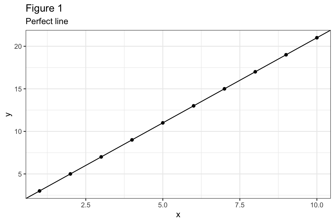
\(|cor(\boldsymbol{x},\boldsymbol{y})| = 1 \iff \boldsymbol{y}= \beta_0 \boldsymbol{1}+ \beta_1 \boldsymbol{x}\) for some \(\beta_0\), \(\beta_1\). See Figure 1.

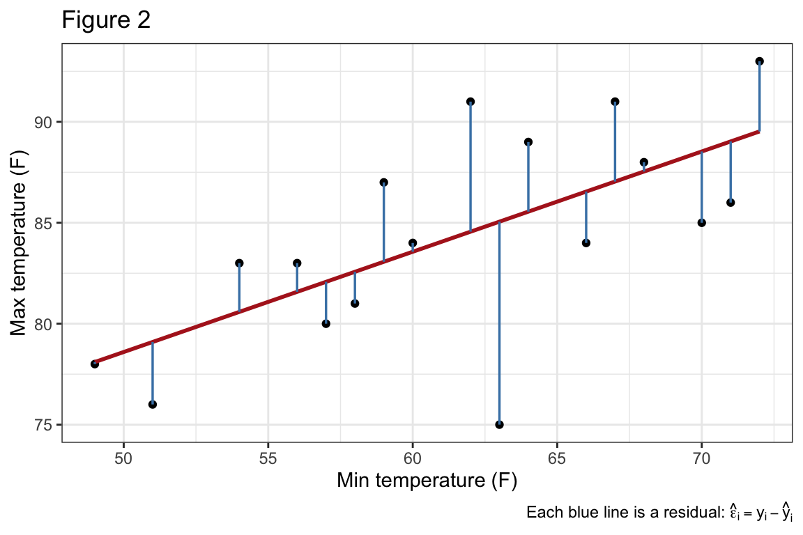
It is more typical that \(|cor(\boldsymbol{x}, \boldsymbol{y})| < 1\), in which case \(\boldsymbol{y}= \beta_0 \boldsymbol{1}+ \beta_1 \boldsymbol{x}+ \boldsymbol{\varepsilon}\), where \(\boldsymbol{\varepsilon}\) is the error vector. See Figure 2 for an example. The observation by observation representation is given by the equation

\[y_i = \beta_0 + \beta_1 x_i + \varepsilon_i.\]

Question: what line, (i.e. what (\(\beta_0, \beta_1\))) provides the “best fit”?

Answer: the set (\(\beta_0, \beta_1\)) that satisfy an objective function.

Definition: objective function

An objective function is some function we want to optimize.

Example 1: least absolute value (LAV) regression

\[ \hat{\beta_0}, \hat{\beta_1} = \operatorname*{arg\,min}_{\beta_0, \beta_1} \sum_{i=1}^n |\varepsilon_i| \]

Example 2: Ordinary least squares (OLS) regression

\[ \hat{\beta_0}, \hat{\beta_1} = \operatorname*{arg\,min}_{\beta_0, \beta_1} \sum_{i=1}^n \varepsilon_i^2 \]

Ordinary least squares (OLS) regression line

\(\sum_{i=1}^n \varepsilon_i^2\) is called the “residual sum of squares” or RSS for short.

\[ \begin{aligned} RSS(\beta_0, \beta_1) &= \sum_{i=1}^n \varepsilon_i^2\\ &= \sum_{i=1}^n (y_i - (\beta_0 + \beta_1 x_i))^2\\ &= (\boldsymbol{y}- (\beta_0 \boldsymbol{1}+ \beta_1 \boldsymbol{x}))^T (\boldsymbol{y}- (\beta_0 \boldsymbol{1}+ \beta_1 \boldsymbol{x}))\\ &= ||(\boldsymbol{y}- (\beta_0 \boldsymbol{1}+ \beta_1 \boldsymbol{x}))||^2 \end{aligned} \]

Definition: OLS estimates

The OLS values of \(\beta_0\), \(\beta_1\) are the values \((\hat{\beta}_0, \hat{\beta}_1)\) that minimize \(RSS(\beta_0, \beta_1)\). Again, in math,

\[ \hat{\beta_0}, \hat{\beta_1} = \operatorname*{arg\,min}_{\beta_0, \beta_1} \sum_{i=1}^n \varepsilon_i^2 \]

Question: How can we find the OLS line?

Answer: (1) Geometry (we’ll do this later); (2) calculus

Computing the OLS estimates using calculus

lm(tmax ~ tmin, data = weather)

Call:
lm(formula = tmax ~ tmin, data = weather)

Coefficients:
(Intercept)         tmin  
    61.1017       0.3729  

• Notice that the RSS is a quadratic (convex) function of \(\beta_0, \beta_1\).

• The global minimum occurs where the derivative (gradient) equals zero.

\[ \begin{aligned} \frac{\partial}{\partial \beta_0} RSS &= -2 \sum (y_i - (\beta_0 + \beta_1 x_i)) = 0\\ \frac{\partial}{\partial \beta_1} RSS &= -2 \sum x_i(y_i - (\beta_0 + \beta_1 x_i)) = 0 \end{aligned} \]

Therefore the OLS values \(\hat{\beta_0}, \hat{\beta_1}\) will satisfy the normal equations,

\[ \begin{align} \sum_{i=1}^n \big(y_i - (\hat{\beta_0} + \hat{\beta_1} x_i)\big) &= 0 \tag{1}\\ \sum_{i=1}^n x_i \big(y_i - (\hat{\beta_0} + \hat{\beta_1} x_i)\big) &= 0 \tag{2} \end{align} \] Question: why are these called the normal equations?

Answer: Let \(\hat{\varepsilon}_i = y_i - \hat{y}_i = y_i - (\hat{\beta_0} + \hat{\beta_1} x_i)\) then,

\[ \begin{aligned} (1) &\implies \sum \hat{\varepsilon}_i = \hat{\boldsymbol{\varepsilon}}\cdot \boldsymbol{1}= 0\\ (2) &\implies \sum x_i \hat{\varepsilon}_i = \boldsymbol{x}^T \hat{\boldsymbol{\varepsilon}}= 0. \end{aligned} \]

In words, the residual vector \(\hat{\boldsymbol{\varepsilon}}\) is normal (orthogonal) to the vectors \(\boldsymbol{1}\) and \(\boldsymbol{x}\).

Exercise

Show that the OLS regression line goes through \(\bar{x}, \bar{y}\). Reminder: \(\bar{x} = \frac{1}{n}\sum x_i\) and \(\bar{y} = \frac{1}{n} \sum y_i\)

Solution

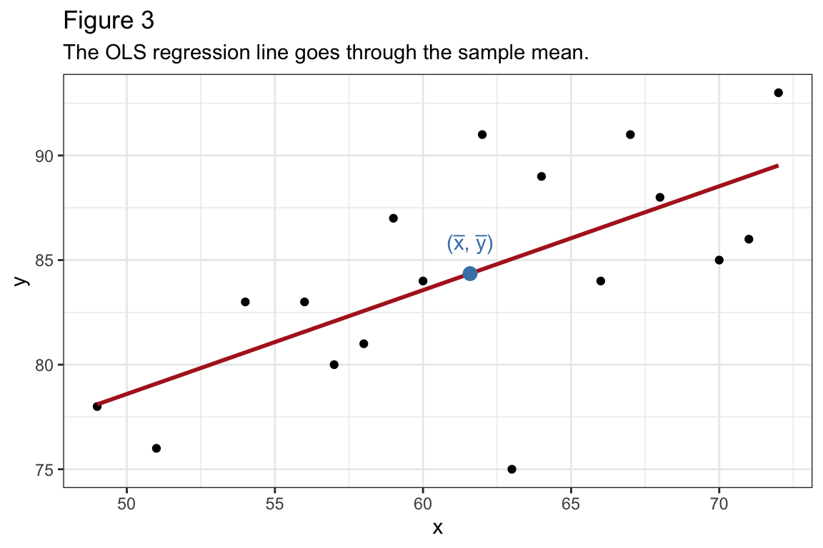
\[ \begin{aligned} (1) \implies &\sum y_i - \sum(\hat{\beta_0} + \hat{\beta_1} x_i) = 0\\ &\sum y_i = \sum(\hat{\beta_0} + \hat{\beta_1} x_i)\\ & n\bar{y} = n \hat{\beta_0} + n \hat{\beta_1} \bar{x}\\ &\bar{y} = \hat{\beta_0} + \hat{\beta_1} \bar{x}. \end{aligned} \] Note the commonly used “trick”:

\(\sum y_i = n \bar{y}\).

Solving the normal equations

\[ \begin{aligned} \text{From (1): } &\sum_{i=1}^n \big(y_i - (\hat{\beta_0} + \hat{\beta_1} x_i)\big) = 0\\ & \bar{y} = \hat{\beta}_0 + \hat{\beta}_1 \bar{x}\\ &\hat{\beta}_0 = \bar{y} - \hat{\beta}_1 \bar{x} \end{aligned} \] Plugging this result into (2):

\[ \begin{aligned} &\sum x_i (y_i - (\hat{\beta}_0 + \hat{\beta}_1 x_i)) = 0\\ &\sum x_i (y_i - \bar{y} + \hat{\beta}_1 \bar{x} - \hat{\beta}_1 x_i) = 0\\ &\sum x_i (y_i - \bar{y}) = \hat{\beta}_1 \sum x_i (x_i - \bar{x}) \text{ }& (*) \end{aligned} \]

Notice the trick:

\[ \begin{aligned} \sum (x_i - \bar{x}) (y_i - \bar{y}) &= \sum x_i (y_i - \bar{y}) - \sum \bar{x}(y_i - \bar{y})\\ &= \sum x_i (y_i - \bar{y}) - \bar{x} (0)\\ &= \sum x_i (y_i - \bar{y}). \end{aligned} \] Similarly,

\[ \begin{aligned} \sum x_i (x_i - \bar{x}) &= \sum (x_i - \bar{x})(x_i - \bar{x})\\ &= \sum (x_i - \bar{x})^2. \end{aligned} \]

Let

\[ \begin{aligned} S_{xx} &= \sum (x_i - \bar{x})^2\\ S_{yy} &= \sum (y_i - \bar{y})^2\\ S_{xy} &= \sum (x_i - \bar{x}) (y_i - \bar{y}) \end{aligned} \] Then \((*)\) above says \(S_{xy} = \hat{\beta}_1 S_{xx}\), implying that the OLS values are

\[ \begin{aligned} \hat{\beta}_0 &= \bar{y} - \hat{\beta}_1 \bar{x}\\ \hat{\beta}_1 &= \frac{S_{xy}}{S_{xx}}. \end{aligned} \]

An important take-away: the slope is closely related to the correlation. Notice

\[ \hat{\beta}_1 = \frac{S_{xy}}{S_{xx}} = \frac{\sum (x_i - \bar{x}) (y_i - \bar{y})}{\sum (x_i - \bar{x})^2} \]

The numerator looks like covariance, or correlation between \(\boldsymbol{x}\) and \(\boldsymbol{y}\). The denominator looks like \(var(\boldsymbol{x})\). If we multiply by the number “1” in a fancy way, the relationship becomes clear,

\[ \begin{aligned} \frac{S_{yy}^{1/2}}{S_{yy}^{1/2}} \cdot \frac{S_{xy}}{S_{xx}^{1/2} S_{xx}^{1/2}} &= \left(\frac{S_{yy}}{S_{xx}}\right)^{1/2} \cdot \frac{S_{xy}}{\left(S_{xx} S_{yy}\right)^{1/2}}\\ &= \left(\frac{S_{yy}}{S_{xx}}\right)^{1/2} \cdot cor(\boldsymbol{x},\boldsymbol{y}) \end{aligned} \]

Summary: what do you need to find \(\hat{\beta}_0, \hat{\beta}_1\)?

• \(\bar{x}\), \(\bar{y}\)
• \(S_{xx}, S_{yy}\)
• \(cor(\boldsymbol{x}, \boldsymbol{y})\)

We can write the fitted regression line in terms of these quantities:

\[ \begin{aligned} \hat{y}_i &= \hat{\beta}_0 + \hat{\beta}_1 x_i\\ &= \bar{y} -\hat{\beta}_1 \bar{x} + \hat{\beta}_1 x_i\\ &= \bar{y} +\hat{\beta}_1 (x_i - \bar{x})\\ &= \bar{y} + \left(S_{yy}/S_{xx} \right)^{1/2} \cdot cor(\boldsymbol{x}, \boldsymbol{y}) \cdot (x_i - \bar{x}) \end{aligned} \]