Correlation and intro to simple linear regresion

library(tidyverse)
library(DT)
 
weather <-
  read_csv("https://sta221-fa25.github.io/data/rdu-weather-history.csv") %>%
  arrange(date)

Learning objectives

By the end of the day you should be able to explain the following concepts:

1. covariance
2. correlation
3. location and scale invariance
4. ordinary least squares

Example

This data set contains Raleigh Durham International Airport weather data pulled from the NOAA web service between September 01 and September 30, 2021. The data were sourced from https://catalog.data.gov/ August 28, 2025.

We’ve recorded 30 observations of two measurements. We are interested in the association between these two measurements.

We’ll call the minimum daily temperature measurement “x” and the maximum daily temperature “y”.

Vocabulary

Variable	Explanation
\(y\)	The outcome variable. Also called “response” or “dependent variable”. In prediction tasks, this is the variable we are interested in predicting.
\(x\)	The predictor. Also called “covariate”, “feature”, or “independent variable”.

How are \(x\) and \(y\) associated?

Scatter plot

Code

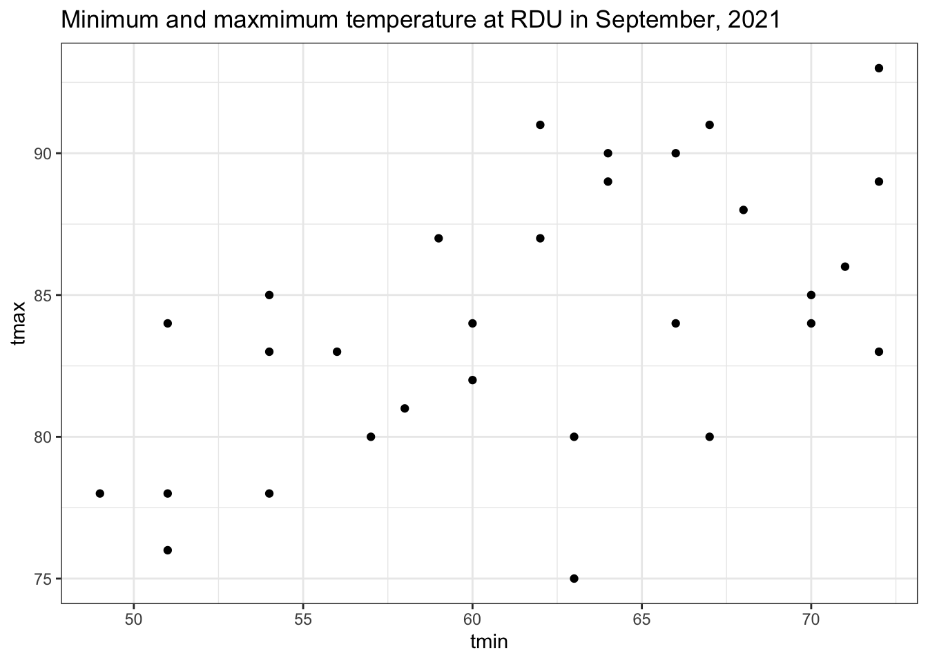
weather %>%
  ggplot(aes(x = tmin, y = tmax)) +
  geom_point() +
  labs(title = "Minimum and maxmimum temperature (F) at RDU in September, 2021") +
  theme_bw()

Notice: visualized this way, each of the thirty data points, \((x_i, y_i)\), is an element of two-dimensional space.

• How would you describe the association?

Definition: covariance

\(cov(x, y) = \frac{1}{n-1}\sum_{i =1}^n (x_i - \bar{x}) (y_i - \bar{y})\) \(^*\)

\(^*\) Note that we divide by \(n-1\) when computing the sample covariance

• \(\bar{x} = \frac{1}{n} \sum x_i\) (mean of x)
• \(\bar{y} = \frac{1}{n} \sum y_i\) (mean of y)

x = weather %>%
  select(tmin) %>%
  pull()
y = weather %>%
  select(tmax) %>%
  pull()

cov(x, y)

[1] 18.68736

sum((x - mean(x)) * (y - mean(y))) / (30 - 1)

[1] 18.68736

• Should the association be the same if the thermometer recording measurements was consistently off by 2 degrees Farenheit?

# compute covariance of true temperature measurement
weather %>%
  mutate(temp_min_true = tmin + 2,
         temp_max_true = tmax + 2) %>%
  summarize(cov(temp_min_true, temp_max_true)) %>%
  pull()

[1] 18.68736

Covariance is location invariant.

• Will the association stay the same if we recorded temperature in celsius?

# compute the covariance between temperature in celsius
weather %>%
  mutate(temp_min_c = (tmin - 32) * 5 / 9,
         temp_max_c = (tmax - 32) * 5 / 9) %>%
  summarize(cov(temp_min_c, temp_max_c)) %>%
  pull()

[1] 5.767703

Covariance is not scale invariant. That is, covariance does depend on the scale of the measurements.

Correlation

Definition: correlation

\(cor(x, y) = \frac{\sum_{i=1}^n (x_i - \bar{x}) (y_i - \bar{y})}{\left(\sum (x_i - \bar{x})^2 \sum (y_i - \bar{y})^2\right)^{1/2}}\)

More concisely, we may write

\(cor(x, y) = \frac{S_{xy}}{S_{xx}^{1/2} S_{yy}^{1/2}}\)

# correlation in Farenheit vs Celsi
# compute the covariance between temperature in celsius
weather %>%
  mutate(temp_min_c = (tmin - 32) * 5 / 9,
         temp_max_c = (tmax - 32) * 5 / 9) %>%
  summarize(cor_F = cor(tmin, tmax), 
            cor_C = cor(temp_min_c, temp_max_c))

# A tibble: 1 × 2
  cor_F cor_C
  <dbl> <dbl>
1 0.554 0.554

Exercise

Show \(cor(x, y) = cor(ax + b, cy + d)\).

Solution

Let \[ \begin{aligned} x^* &= ax_i + b,\\ y^* &= cx_i + d, \end{aligned} \]

then we want to prove that \(cor(x, y) = cor(x^*, y^*)\).

\[ \begin{aligned} cor(x^*, y^*) &= \frac{\sum(ax_i + b - a\bar{x} - b)(cy_i + d - c\bar{y} - d)}{\sqrt{ \sum (ax_i + b - a\bar{x} - b)^2 \sum (cy_i + d - c\bar{y} - d)^2 } }\\ &= \frac{ac \sum(x_i -\bar{x})(y_i - \bar{y})}{ ac \sqrt{\sum (ax_i + b - a\bar{x} - b)^2 \sum (cy_i + d - c\bar{y} - d)^2 } }\\ &= \frac{ S_{xy}}{\sqrt{S_{xx} S_{yy}} } \end{aligned} \]

Correlation is location and scale invariant!

Additional facts about correlation:

Fact 1

• Correlation is not invariant to monotone transformations of the data

Definition: monotone

\(g\) is a monotonic function iff \(x \leq y\) implies \(g(x) \leq g(y)\)

Exercise

Show by example that correlation is not invariant to monotonic transformations.

Solution

set.seed(221)
x = c(1:10) 
logx = log(x)
y = rnorm(10)
cor(x, y)

[1] -0.1757986

cor(logx, y)

[1] -0.2686214

Fact 2

• Correlation is not robust to outliers

Example 1

set.seed(221)
x = c(1:5)
y= x + rnorm(5)
plot(x, y)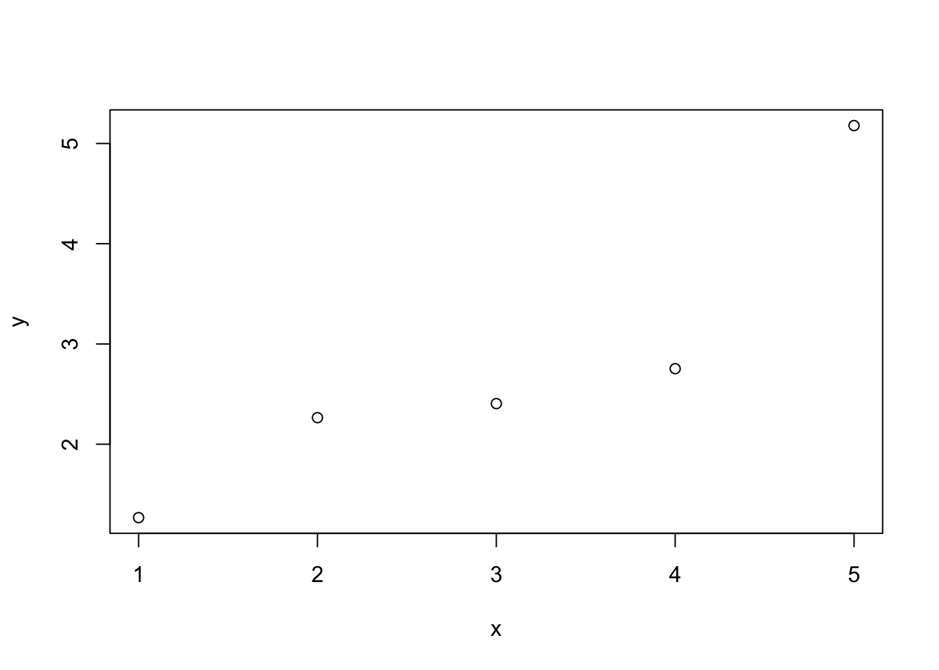

cor(x, y)

[1] 0.9042223

Example 2

x2 = c(x, 0)
y2 = c(y, 20)
plot(x2, y2)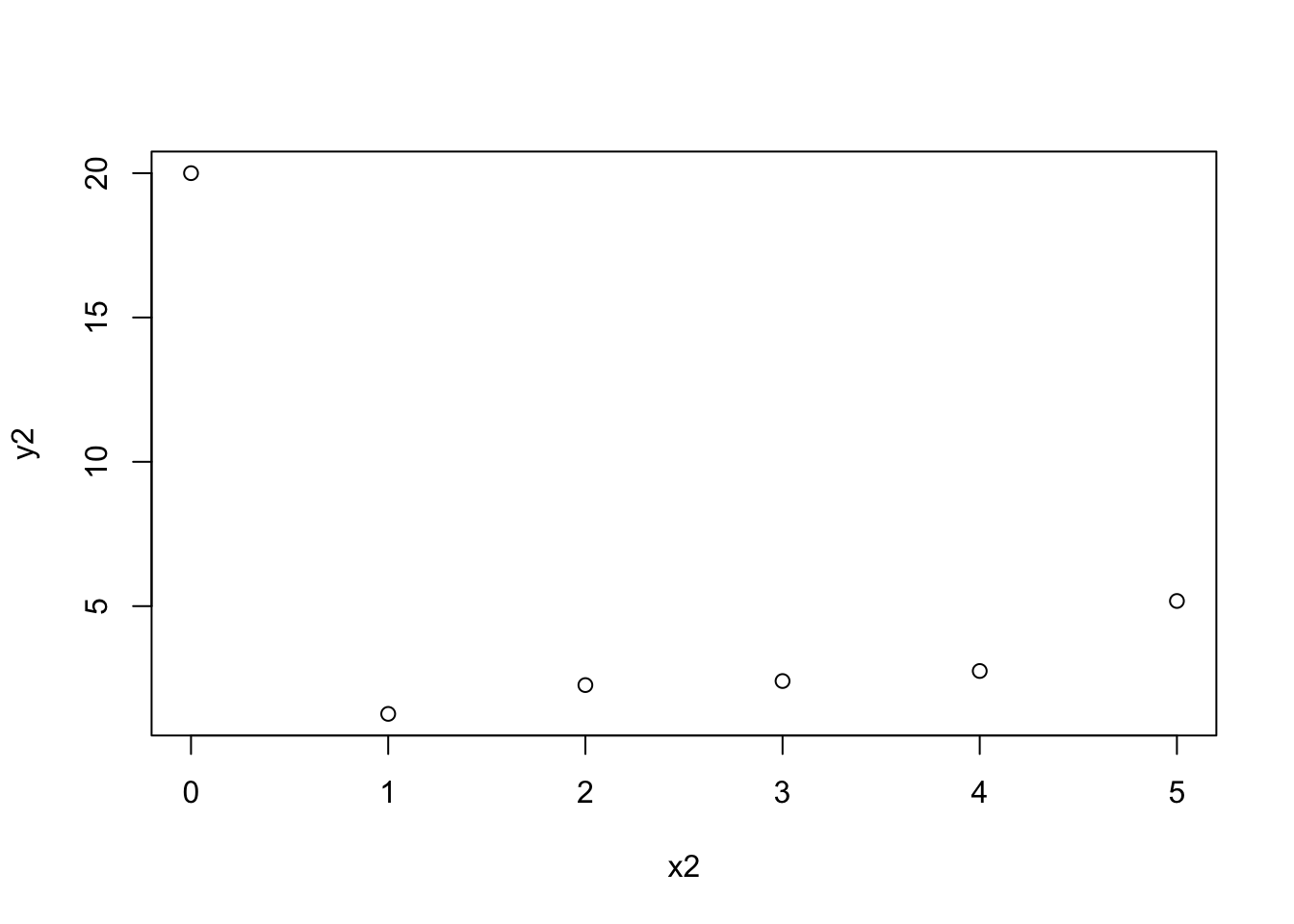

cor(x2, y2)

[1] -0.5195233

Fact 3

Correlation is bounded between -1 and 1.

Exercise

Show that \(|cor(x, y)| \leq 1\)

Solution

Cauchy-Schwarz inequality:

Let \(u\) and \(v\) be vectors of dimension \(n\), then

\[ |u^T v|^2 \leq (u^Tu) (v^Tv). \] To prove that \(\|cor(x,y)\| \leq 1\), let \(u = x - \bar{x}\) and let \(v = y - \bar{y}\).

Important

Notice that the dimension of a vector inner product, e.g. \(u^Tv\) is \(1 \times 1\), in other words, it is a “scalar”, a number.

Fact 4

• correlation is a measure of linear association

Example 1

x = -10:10
y = x^2
plot(x, y)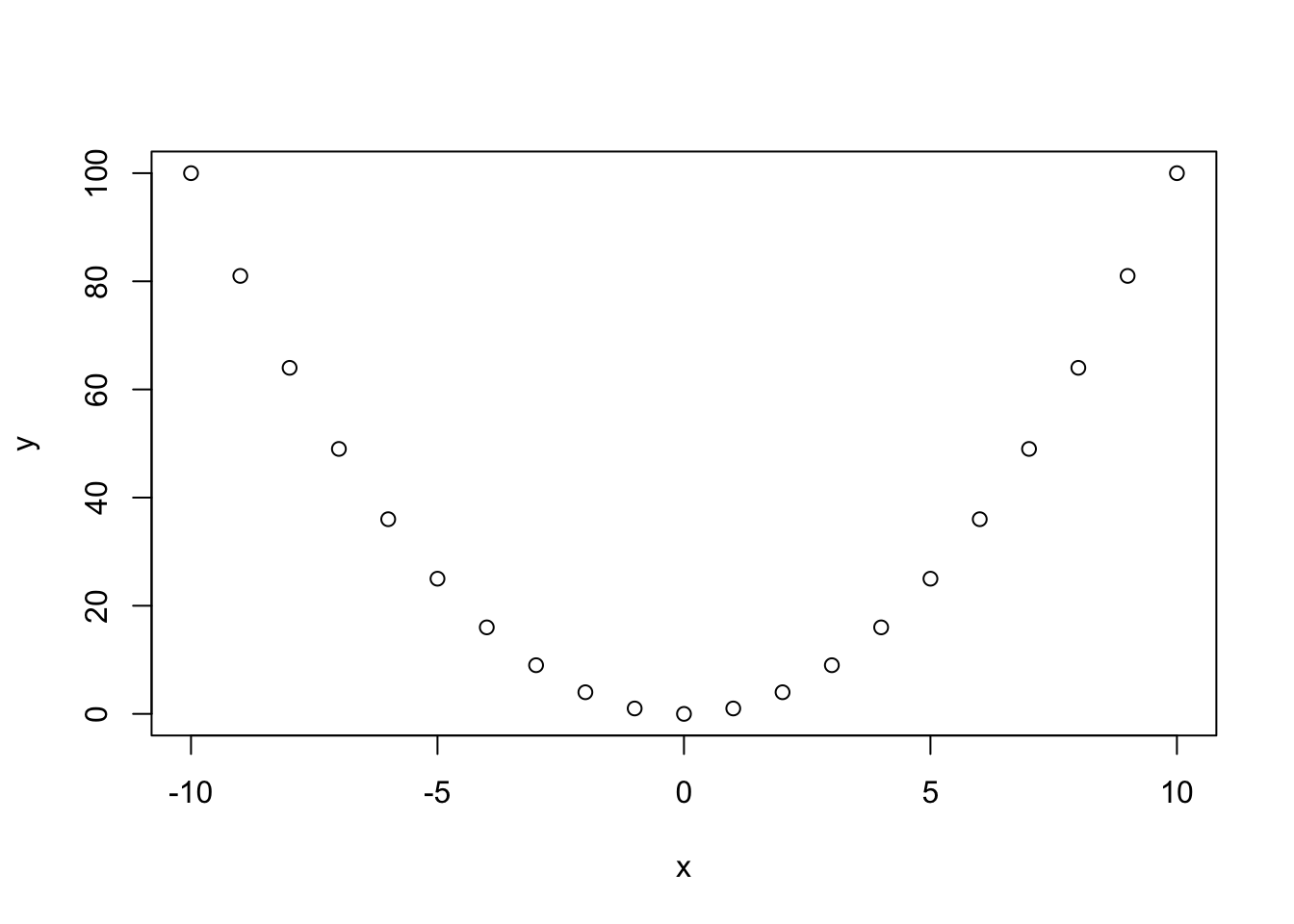

cor(x, y) 

[1] -4.786989e-17

Example 2

x = -10:10
y = x
plot(x, y)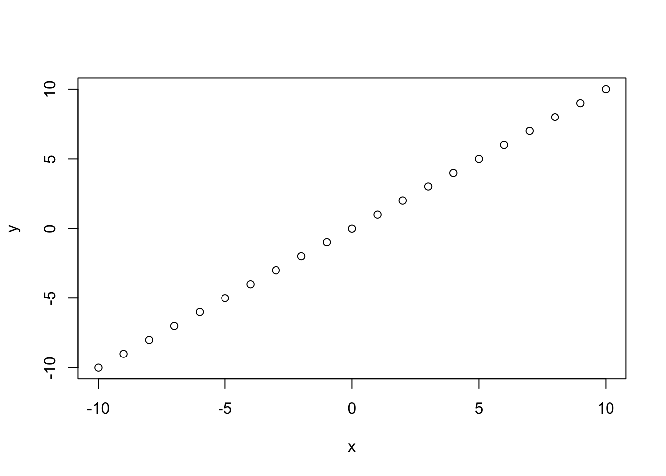

cor(x, y)

[1] 1

Since correlation is related to a linear relationship between the data, strong correlation implies that

\[ y_i = \beta_0 + \beta_1 x_i + \epsilon_i \]

Exercise

Check out the interactive regression web app here:

https://seeing-theory.brown.edu/regression-analysis/index.html#section1

Nomenclature of simple linear regression

Symbol	Description
\(y\)	The response variable. Also called the “outcome” or “dependent variable”.
\(x\)	A covariate. Also called the “predictor”, “feature” or “independent variable”.
\(\beta_0, \beta_1\)	These are population parameters, i.e. fixed and unknown constants.
\(\hat{\beta}_0, \hat{\beta}_1\)	Estimates of \(\beta_0, \beta_1\) based on a sample.
\(\hat{y}\)	The prediction outcome. \(\hat{y} = \hat{\beta_0} + \hat{\beta_1} x\). May also be referred to as the “fitted regression model”.
\(\epsilon\)	The error. Defined by the regression equation: \(\epsilon = y - \beta_0 - \beta_1 x\).
\(\hat{\epsilon}\) or \(e\)	The residual, i.e. the difference between the outcome and the fitted model. Defined as \(y - \hat{y}\), or equivalently, \(y - \hat{\beta_0} - \hat{\beta_1}x\)